


COMPOSITION
-
HuggingFace ai-comic-factory – a FREE AI Comic Book Creator
Read more: HuggingFace ai-comic-factory – a FREE AI Comic Book Creatorhttps://huggingface.co/spaces/jbilcke-hf/ai-comic-factory

this is the epic story of a group of talented digital artists trying to overcame daily technical challenges to achieve incredibly photorealistic projects of monsters and aliens


DESIGN


COLOR
-
Weta Digital – Manuka Raytracer and Gazebo GPU renderers – pipeline
Read more: Weta Digital – Manuka Raytracer and Gazebo GPU renderers – pipelinehttps://jo.dreggn.org/home/2018_manuka.pdf
http://www.fxguide.com/featured/manuka-weta-digitals-new-renderer/

The Manuka rendering architecture has been designed in the spirit of the classic reyes rendering architecture. In its core, reyes is based on stochastic rasterisation of micropolygons, facilitating depth of field, motion blur, high geometric complexity,and programmable shading.
This is commonly achieved with Monte Carlo path tracing, using a paradigm often called shade-on-hit, in which the renderer alternates tracing rays with running shaders on the various ray hits. The shaders take the role of generating the inputs of the local material structure which is then used bypath sampling logic to evaluate contributions and to inform what further rays to cast through the scene.
Over the years, however, the expectations have risen substantially when it comes to image quality. Computing pictures which are indistinguishable from real footage requires accurate simulation of light transport, which is most often performed using some variant of Monte Carlo path tracing. Unfortunately this paradigm requires random memory accesses to the whole scene and does not lend itself well to a rasterisation approach at all.
Manuka is both a uni-directional and bidirectional path tracer and encompasses multiple importance sampling (MIS). Interestingly, and importantly for production character skin work, it is the first major production renderer to incorporate spectral MIS in the form of a new ‘Hero Spectral Sampling’ technique, which was recently published at Eurographics Symposium on Rendering 2014.
Manuka propose a shade-before-hit paradigm in-stead and minimise I/O strain (and some memory costs) on the system, leveraging locality of reference by running pattern generation shaders before we execute light transport simulation by path sampling, “compressing” any bvh structure as needed, and as such also limiting duplication of source data.
The difference with reyes is that instead of baking colors into the geometry like in Reyes, manuka bakes surface closures. This means that light transport is still calculated with path tracing, but all texture lookups etc. are done up-front and baked into the geometry.The main drawback with this method is that geometry has to be tessellated to its highest, stable topology before shading can be evaluated properly. As such, the high cost to first pixel. Even a basic 4 vertices square becomes a much more complex model with this approach.

Manuka use the RenderMan Shading Language (rsl) for programmable shading [Pixar Animation Studios 2015], but we do not invoke rsl shaders when intersecting a ray with a surface (often called shade-on-hit). Instead, we pre-tessellate and pre-shade all the input geometry in the front end of the renderer.
This way, we can efficiently order shading computations to sup-port near-optimal texture locality, vectorisation, and parallelism. This system avoids repeated evaluation of shaders at the same surface point, and presents a minimal amount of memory to be accessed during light transport time. An added benefit is that the acceleration structure for ray tracing (abounding volume hierarchy, bvh) is built once on the final tessellated geometry, which allows us to ray trace more efficiently than multi-level bvhs and avoids costly caching of on-demand tessellated micropolygons and the associated scheduling issues.For the shading reasons above, in terms of AOVs, the studio approach is to succeed at combining complex shading with ray paths in the render rather than pass a multi-pass render to compositing.
For the Spectral Rendering component. The light transport stage is fully spectral, using a continuously sampled wavelength which is traced with each path and used to apply the spectral camera sensitivity of the sensor. This allows for faithfully support any degree of observer metamerism as the camera footage they are intended to match as well as complex materials which require wavelength dependent phenomena such as diffraction, dispersion, interference, iridescence, or chromatic extinction and Rayleigh scattering in participating media.
As opposed to the original reyes paper, we use bilinear interpolation of these bsdf inputs later when evaluating bsdfs per pathv ertex during light transport4. This improves temporal stability of geometry which moves very slowly with respect to the pixel raster
In terms of the pipeline, everything rendered at Weta was already completely interwoven with their deep data pipeline. Manuka very much was written with deep data in mind. Here, Manuka not so much extends the deep capabilities, rather it fully matches the already extremely complex and powerful setup Weta Digital already enjoy with RenderMan. For example, an ape in a scene can be selected, its ID is available and a NUKE artist can then paint in 3D say a hand and part of the way up the neutral posed ape.
We called our system Manuka, as a respectful nod to reyes: we had heard a story froma former ILM employee about how reyes got its name from how fond the early Pixar people were of their lunches at Point Reyes, and decided to name our system after our surrounding natural environment, too. Manuka is a kind of tea tree very common in New Zealand which has very many very small leaves, in analogy to micropolygons ina tree structure for ray tracing. It also happens to be the case that Weta Digital’s main site is on Manuka Street.

-
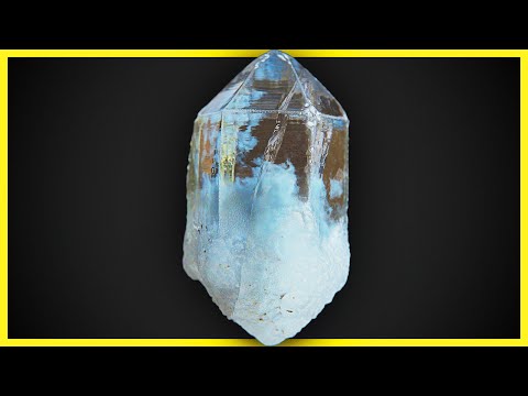
Tim Kang – calibrated white light values in sRGB color space
Read more: Tim Kang – calibrated white light values in sRGB color space8bit sRGB encoded
2000K 255 139 22
2700K 255 172 89
3000K 255 184 109
3200K 255 190 122
4000K 255 211 165
4300K 255 219 178
D50 255 235 205
D55 255 243 224
D5600 255 244 227
D6000 255 249 240
D65 255 255 255
D10000 202 221 255
D20000 166 196 2558bit Rec709 Gamma 2.4
2000K 255 145 34
2700K 255 177 97
3000K 255 187 117
3200K 255 193 129
4000K 255 214 170
4300K 255 221 182
D50 255 236 208
D55 255 243 226
D5600 255 245 229
D6000 255 250 241
D65 255 255 255
D10000 204 222 255
D20000 170 199 2558bit Display P3 encoded
2000K 255 154 63
2700K 255 185 109
3000K 255 195 127
3200K 255 201 138
4000K 255 219 176
4300K 255 225 187
D50 255 239 212
D55 255 245 228
D5600 255 246 231
D6000 255 251 242
D65 255 255 255
D10000 208 223 255
D20000 175 199 25510bit Rec2020 PQ (100 nits)
2000K 520 435 273
2700K 520 466 358
3000K 520 475 384
3200K 520 480 399
4000K 520 495 446
4300K 520 500 458
D50 520 510 482
D55 520 514 497
D5600 520 514 500
D6000 520 517 509
D65 520 520 520
D10000 479 489 520
D20000 448 464 520
-
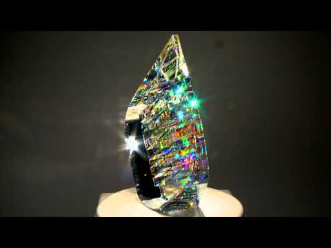
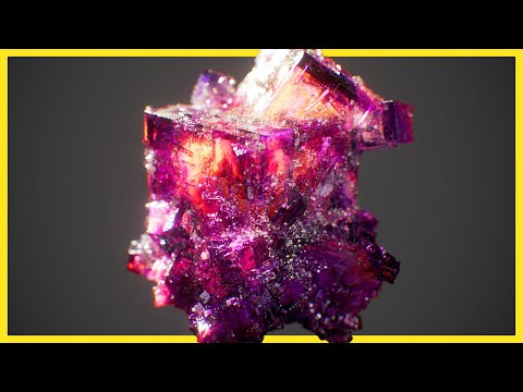
Björn Ottosson – OKlch color space
Read more: Björn Ottosson – OKlch color spaceBjörn Ottosson proposed OKlch in 2020 to create a color space that can closely mimic how color is perceived by the human eye, predicting perceived lightness, chroma, and hue.
The OK in OKLCH stands for Optimal Color.
- L: Lightness (the perceived brightness of the color)
- C: Chroma (the intensity or saturation of the color)
- H: Hue (the actual color, such as red, blue, green, etc.)

Also read:
-
Björn Ottosson – How software gets color wrong
Read more: Björn Ottosson – How software gets color wronghttps://bottosson.github.io/posts/colorwrong/
Most software around us today are decent at accurately displaying colors. Processing of colors is another story unfortunately, and is often done badly.
To understand what the problem is, let’s start with an example of three ways of blending green and magenta:
- Perceptual blend – A smooth transition using a model designed to mimic human perception of color. The blending is done so that the perceived brightness and color varies smoothly and evenly.
- Linear blend – A model for blending color based on how light behaves physically. This type of blending can occur in many ways naturally, for example when colors are blended together by focus blur in a camera or when viewing a pattern of two colors at a distance.
- sRGB blend – This is how colors would normally be blended in computer software, using sRGB to represent the colors.

Let’s look at some more examples of blending of colors, to see how these problems surface more practically. The examples use strong colors since then the differences are more pronounced. This is using the same three ways of blending colors as the first example.

Instead of making it as easy as possible to work with color, most software make it unnecessarily hard, by doing image processing with representations not designed for it. Approximating the physical behavior of light with linear RGB models is one easy thing to do, but more work is needed to create image representations tailored for image processing and human perception.
Also see:


LIGHTING
-
Custom bokeh in a raytraced DOF render
Read more: Custom bokeh in a raytraced DOF render

To achieve a custom pinhole camera effect with a custom bokeh in Arnold Raytracer, you can follow these steps:
- Set the render camera with a focal length around 50 (or as needed)
- Set the F-Stop to a high value (e.g., 22).
- Set the focus distance as you require
- Turn on DOF
- Place a plane a few cm in front of the camera.
- Texture the plane with a transparent shape at the center of it. (Transmission with no specular roughness)
-
HDRI Median Cut plugin
Read more: HDRI Median Cut pluginwww.hdrlabs.com/picturenaut/plugins.html

Note. The Median Cut algorithm is typically used for color quantization, which involves reducing the number of colors in an image while preserving its visual quality. It doesn’t directly provide a way to identify the brightest areas in an image. However, if you’re interested in identifying the brightest areas, you might want to look into other methods like thresholding, histogram analysis, or edge detection, through openCV for example.
Here is an openCV example:
# bottom left coordinates = 0,0 import numpy as np import cv2 # Load the HDR or EXR image image = cv2.imread('your_image_path.exr', cv2.IMREAD_UNCHANGED) # Load as-is without modification # Calculate the luminance from the HDR channels (assuming RGB format) luminance = np.dot(image[..., :3], [0.299, 0.587, 0.114]) # Set a threshold value based on estimated EV threshold_value = 2.4 # Estimated threshold value based on 4.8 EV # Apply the threshold to identify bright areas # Theluminancearray contains the calculated luminance values for each pixel in the image. # Thethreshold_valueis a user-defined value that represents a cutoff point, separating "bright" and "dark" areas in terms of perceived luminance.thresholded = (luminance > threshold_value) * 255 # Convert the thresholded image to uint8 for contour detection thresholded = thresholded.astype(np.uint8) # Find contours of the bright areas contours, _ = cv2.findContours(thresholded, cv2.RETR_EXTERNAL, cv2.CHAIN_APPROX_SIMPLE) # Create a list to store the bounding boxes of bright areas bright_areas = [] # Iterate through contours and extract bounding boxes for contour in contours: x, y, w, h = cv2.boundingRect(contour) # Adjust y-coordinate based on bottom-left origin y_bottom_left_origin = image.shape[0] - (y + h) bright_areas.append((x, y_bottom_left_origin, x + w, y_bottom_left_origin + h)) # Store as (x1, y1, x2, y2) # Print the identified bright areas print("Bright Areas (x1, y1, x2, y2):") for area in bright_areas: print(area)More details
Luminance and Exposure in an EXR Image:
- An EXR (Extended Dynamic Range) image format is often used to store high dynamic range (HDR) images that contain a wide range of luminance values, capturing both dark and bright areas.
- Luminance refers to the perceived brightness of a pixel in an image. In an RGB image, luminance is often calculated using a weighted sum of the red, green, and blue channels, where different weights are assigned to each channel to account for human perception.
- In an EXR image, the pixel values can represent radiometrically accurate scene values, including actual radiance or irradiance levels. These values are directly related to the amount of light emitted or reflected by objects in the scene.
The luminance line is calculating the luminance of each pixel in the image using a weighted sum of the red, green, and blue channels. The three float values [0.299, 0.587, 0.114] are the weights used to perform this calculation.
These weights are based on the concept of luminosity, which aims to approximate the perceived brightness of a color by taking into account the human eye’s sensitivity to different colors. The values are often derived from the NTSC (National Television System Committee) standard, which is used in various color image processing operations.
Here’s the breakdown of the float values:
- 0.299: Weight for the red channel.
- 0.587: Weight for the green channel.
- 0.114: Weight for the blue channel.
The weighted sum of these channels helps create a grayscale image where the pixel values represent the perceived brightness. This technique is often used when converting a color image to grayscale or when calculating luminance for certain operations, as it takes into account the human eye’s sensitivity to different colors.
For the threshold, remember that the exact relationship between EV values and pixel values can depend on the tone-mapping or normalization applied to the HDR image, as well as the dynamic range of the image itself.
To establish a relationship between exposure and the threshold value, you can consider the relationship between linear and logarithmic scales:
- Linear and Logarithmic Scales:
- Exposure values in an EXR image are often represented in logarithmic scales, such as EV (exposure value). Each increment in EV represents a doubling or halving of the amount of light captured.
- Threshold values for luminance thresholding are usually linear, representing an actual luminance level.
- Conversion Between Scales:
- To establish a mathematical relationship, you need to convert between the logarithmic exposure scale and the linear threshold scale.
- One common method is to use a power function. For instance, you can use a power function to convert EV to a linear intensity value.
threshold_value = base_value * (2 ** EV)Here,
EVis the exposure value,base_valueis a scaling factor that determines the relationship between EV and threshold_value, and2 ** EVis used to convert the logarithmic EV to a linear intensity value. - Choosing the Base Value:
- The
base_valuefactor should be determined based on the dynamic range of your EXR image and the specific luminance values you are dealing with. - You may need to experiment with different values of
base_valueto achieve the desired separation of bright areas from the rest of the image.
- The
Let’s say you have an EXR image with a dynamic range of 12 EV, which is a common range for many high dynamic range images. In this case, you want to set a threshold value that corresponds to a certain number of EV above the middle gray level (which is often considered to be around 0.18).
Here’s an example of how you might determine a
base_valueto achieve this:# Define the dynamic range of the image in EV dynamic_range = 12 # Choose the desired number of EV above middle gray for thresholding desired_ev_above_middle_gray = 2 # Calculate the threshold value based on the desired EV above middle gray threshold_value = 0.18 * (2 ** (desired_ev_above_middle_gray / dynamic_range)) print("Threshold Value:", threshold_value) -
IES Light Profiles and editing software
Read more: IES Light Profiles and editing softwarehttp://www.derekjenson.com/3d-blog/ies-light-profiles
https://ieslibrary.com/en/browse#ies
https://leomoon.com/store/shaders/ies-lights-pack
https://docs.arnoldrenderer.com/display/a5afmug/ai+photometric+light
IES profiles are useful for creating life-like lighting, as they can represent the physical distribution of light from any light source.
The IES format was created by the Illumination Engineering Society, and most lighting manufacturers provide IES profile for the lights they manufacture.


-
Unity 3D resources
Read more: Unity 3D resources
http://answers.unity3d.com/questions/12321/how-can-i-start-learning-unity-fast-list-of-tutori.html
If you have no previous experience with Unity, start with these six video tutorials which give a quick overview of the Unity interface and some important features http://unity3d.com/support/documentation/video/
-
PTGui 13 beta adds control through a Patch Editor
Read more: PTGui 13 beta adds control through a Patch EditorAdditions:
- Patch Editor (PTGui Pro)
- DNG output
- Improved RAW / DNG handling
- JPEG 2000 support
- Performance improvements

-
Magnific.ai Relight – change the entire lighting of a scene
Read more: Magnific.ai Relight – change the entire lighting of a scene
It’s a new Magnific spell that allows you to change the entire lighting of a scene and, optionally, the background with just:
1/ A prompt OR
2/ A reference image OR
3/ A light map (drawing your own lights)https://x.com/javilopen/status/1805274155065176489


COLLECTIONS
| Featured AI
| Design And Composition
| Explore posts
POPULAR SEARCHES
unreal | pipeline | virtual production | free | learn | photoshop | 360 | macro | google | nvidia | resolution | open source | hdri | real-time | photography basics | nuke
FEATURED POSTS
Social Links
DISCLAIMER – Links and images on this website may be protected by the respective owners’ copyright. All data submitted by users through this site shall be treated as freely available to share.
