Depth of field is the range within which focusing is resolved in a photo.
Aperture has a huge affect on to the depth of field.
Changing the f-stops (f/#) of a lens will change aperture and as such the DOF.
f-stops are a just certain number which is telling you the size of the aperture. That’s how f-stop is related to aperture (and DOF).
If you increase f-stops, it will increase DOF, the area in focus (and decrease the aperture). On the other hand, decreasing the f-stop it will decrease DOF (and increase the aperture).
The red cone in the figure is an angular representation of the resolution of the system. Versus the dotted lines, which indicate the aperture coverage. Where the lines of the two cones intersect defines the total range of the depth of field.
This image explains why the longer the depth of field, the greater the range of clarity.
Size. Mr. White (Harvey Keitel) on the right. Focus. He’s one of the two objects in focus. Lighting. Mr. White is large and in focus and Mr. Pink (Steve Buscemi) is highlighted by a shaft of light. Color. Both are black and white but the read on Mr. White’s shirt now really stands out.
” In this video, I utilized artificial intelligence to generate an animated music video for the song Canvas by Resonate. This tool allows anyone to generate beautiful images using only text as the input. My question was, what if I used song lyrics as input to the AI, can I make perfect music synchronized videos automatically with the push of a button? Let me know how you think the AI did in this visual interpretation of the song.
After getting caught up in the excitement around DALL·E2 (latest and greatest AI system, it’s INSANE), I searched for any way I could use similar image generation for music synchronization. Since DALL·E2 is not available to the public yet, my search led me to VQGAN + CLIP (Vector Quantized Generative Adversarial Network and Contrastive Language–Image Pre-training), before settling more specifically on Disco Diffusion V5.2 Turbo. If you don’t know what any of these words or acronyms mean, don’t worry, I was just as confused when I first started learning about this technology. I believe we’re reaching a turning point where entire industries are about to shift in reaction to this new process (which is essentially magic!).
This page compares images rendered in Arnold using spectral rendering and different sets of colourspace primaries: Rec.709, Rec.2020, ACES and DCI-P3. The SPD data for the GretagMacbeth Color Checker are the measurements of Noburu Ohta, taken from Mansencal, Mauderer and Parsons (2014) colour-science.org.
Björn Ottosson proposed OKlch in 2020 to create a color space that can closely mimic how color is perceived by the human eye, predicting perceived lightness, chroma, and hue.
The OK in OKLCH stands for Optimal Color.
L: Lightness (the perceived brightness of the color)
C: Chroma (the intensity or saturation of the color)
H: Hue (the actual color, such as red, blue, green, etc.)
Colour is an open-source Python package providing a comprehensive number of algorithms and datasets for colour science. It is freely available under the BSD-3-Clause terms.
This paper presents an introduction to the color pipelines behind modern feature-film visual-effects and animation.
Authored by Jeremy Selan, and reviewed by the members of the VES Technology Committee including Rob Bredow, Dan Candela, Nick Cannon, Paul Debevec, Ray Feeney, Andy Hendrickson, Gautham Krishnamurti, Sam Richards, Jordan Soles, and Sebastian Sylwan.
Supported by LG, Philips, Panasonic and Sony sell the OLED system TVs. OLED stands for “organic light emitting diode.” It is a fundamentally different technology from LCD, the major type of TV today. OLED is “emissive,” meaning the pixels emit their own light.
Samsung is branding its best TVs with a new acronym: “QLED” QLED (according to Samsung) stands for “quantum dot LED TV.” It is a variation of the common LED LCD, adding a quantum dot film to the LCD “sandwich.” QLED, like LCD, is, in its current form, “transmissive” and relies on an LED backlight.
OLED is the only technology capable of absolute blacks and extremely bright whites on a per-pixel basis. LCD definitely can’t do that, and even the vaunted, beloved, dearly departed plasma couldn’t do absolute blacks.
QLED, as an improvement over OLED, significantly improves the picture quality. QLED can produce an even wider range of colors than OLED, which says something about this new tech. QLED is also known to produce up to 40% higher luminance efficiency than OLED technology. Further, many tests conclude that QLED is far more efficient in terms of power consumption than its predecessor, OLED.
“The Color Rendering Index is a measurement of how faithfully a light source reveals the colors of whatever it illuminates, it describes the ability of a light source to reveal the color of an object, as compared to the color a natural light source would provide. The highest possible CRI is 100. A CRI of 100 generally refers to a perfect black body, like a tungsten light source or the sun. ”
In the retina, photoreceptors, bipolar cells, and horizontal cells work together to process visual information before it reaches the brain. Here’s how each cell type contributes to vision:
DISCLAIMER – Links and images on this website may be protected by the respective owners’ copyright. All data submitted by users through this site shall be treated as freely available to share.