COMPOSITION
-
Composition – How to make a slow motion shot
Read more: Composition – How to make a slow motion shothttp://www.slomovideo.com/slowhow.html
Slow motion cinematography is the result of playing back frames for a longer duration than they were exposed. For example, if you expose 240 frames of film in one second, then play them back at 24 fps, the resulting movie is 10 times longer (slower) than the original filmed event….
DESIGN
-
VQGAN + CLIP AI made Music Video for the song Canvas by Resonate
Read more: VQGAN + CLIP AI made Music Video for the song Canvas by Resonate” In this video, I utilized artificial intelligence to generate an animated music video for the song Canvas by Resonate. This tool allows anyone to generate beautiful images using only text as the input. My question was, what if I used song lyrics as input to the AI, can I make perfect music synchronized videos automatically with the push of a button? Let me know how you think the AI did in this visual interpretation of the song.
After getting caught up in the excitement around DALL·E2 (latest and greatest AI system, it’s INSANE), I searched for any way I could use similar image generation for music synchronization. Since DALL·E2 is not available to the public yet, my search led me to VQGAN + CLIP (Vector Quantized Generative Adversarial Network and Contrastive Language–Image Pre-training), before settling more specifically on Disco Diffusion V5.2 Turbo. If you don’t know what any of these words or acronyms mean, don’t worry, I was just as confused when I first started learning about this technology. I believe we’re reaching a turning point where entire industries are about to shift in reaction to this new process (which is essentially magic!).
DoodleChaos”
-
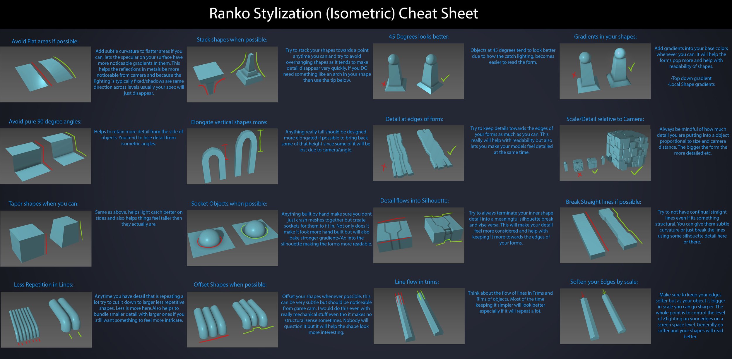
Ranko Prozo – Modelling design tips
Read more: Ranko Prozo – Modelling design tipsEvery Project I work on I always create a stylization Cheat sheet. Every project is unique but some principles carry over no matter what. This is a sheet I use a lot when I work on isometric stylized projects to help keep my assets consistent and interesting. None of these concepts are my own, just lots of tips I learned over the years. I have also added this to a page on my website, will continue to update with more tips and tricks, just need time to compile it all :)
COLOR
-
The Forbidden colors – Red-Green & Blue-Yellow: The Stunning Colors You Can’t See
Read more: The Forbidden colors – Red-Green & Blue-Yellow: The Stunning Colors You Can’t Seewww.livescience.com/17948-red-green-blue-yellow-stunning-colors.html
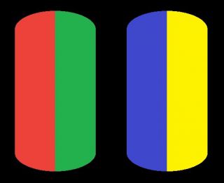
While the human eye has red, green, and blue-sensing cones, those cones are cross-wired in the retina to produce a luminance channel plus a red-green and a blue-yellow channel, and it’s data in that color space (known technically as “LAB”) that goes to the brain. That’s why we can’t perceive a reddish-green or a yellowish-blue, whereas such colors can be represented in the RGB color space used by digital cameras.
https://en.rockcontent.com/blog/the-use-of-yellow-in-data-design
The back of the retina is covered in light-sensitive neurons known as cone cells and rod cells. There are three types of cone cells, each sensitive to different ranges of light. These ranges overlap, but for convenience the cones are referred to as blue (short-wavelength), green (medium-wavelength), and red (long-wavelength). The rod cells are primarily used in low-light situations, so we’ll ignore those for now.
When light enters the eye and hits the cone cells, the cones get excited and send signals to the brain through the visual cortex. Different wavelengths of light excite different combinations of cones to varying levels, which generates our perception of color. You can see that the red cones are most sensitive to light, and the blue cones are least sensitive. The sensitivity of green and red cones overlaps for most of the visible spectrum.

Here’s how your brain takes the signals of light intensity from the cones and turns it into color information. To see red or green, your brain finds the difference between the levels of excitement in your red and green cones. This is the red-green channel.
To get “brightness,” your brain combines the excitement of your red and green cones. This creates the luminance, or black-white, channel. To see yellow or blue, your brain then finds the difference between this luminance signal and the excitement of your blue cones. This is the yellow-blue channel.
From the calculations made in the brain along those three channels, we get four basic colors: blue, green, yellow, and red. Seeing blue is what you experience when low-wavelength light excites the blue cones more than the green and red.
Seeing green happens when light excites the green cones more than the red cones. Seeing red happens when only the red cones are excited by high-wavelength light.
Here’s where it gets interesting. Seeing yellow is what happens when BOTH the green AND red cones are highly excited near their peak sensitivity. This is the biggest collective excitement that your cones ever have, aside from seeing pure white.
Notice that yellow occurs at peak intensity in the graph to the right. Further, the lens and cornea of the eye happen to block shorter wavelengths, reducing sensitivity to blue and violet light.
-
Black Body color aka the Planckian Locus curve for white point eye perception
Read more: Black Body color aka the Planckian Locus curve for white point eye perceptionhttp://en.wikipedia.org/wiki/Black-body_radiation
Black-body radiation is the type of electromagnetic radiation within or surrounding a body in thermodynamic equilibrium with its environment, or emitted by a black body (an opaque and non-reflective body) held at constant, uniform temperature. The radiation has a specific spectrum and intensity that depends only on the temperature of the body.
A black-body at room temperature appears black, as most of the energy it radiates is infra-red and cannot be perceived by the human eye. At higher temperatures, black bodies glow with increasing intensity and colors that range from dull red to blindingly brilliant blue-white as the temperature increases.
The Black Body Ultraviolet Catastrophe Experiment
In photography, color temperature describes the spectrum of light which is radiated from a “blackbody” with that surface temperature. A blackbody is an object which absorbs all incident light — neither reflecting it nor allowing it to pass through.
The Sun closely approximates a black-body radiator. Another rough analogue of blackbody radiation in our day to day experience might be in heating a metal or stone: these are said to become “red hot” when they attain one temperature, and then “white hot” for even higher temperatures. Similarly, black bodies at different temperatures also have varying color temperatures of “white light.”
Despite its name, light which may appear white does not necessarily contain an even distribution of colors across the visible spectrum.
Although planets and stars are neither in thermal equilibrium with their surroundings nor perfect black bodies, black-body radiation is used as a first approximation for the energy they emit. Black holes are near-perfect black bodies, and it is believed that they emit black-body radiation (called Hawking radiation), with a temperature that depends on the mass of the hole.
-
Akiyoshi Kitaoka – Surround biased illumination perception
Read more: Akiyoshi Kitaoka – Surround biased illumination perceptionhttps://x.com/AkiyoshiKitaoka/status/1798705648001327209
The left face appears whitish and the right one blackish, but they are made up of the same luminance.
https://community.wolfram.com/groups/-/m/t/3191015
Illusory staircase Gelb effect
https://www.psy.ritsumei.ac.jp/akitaoka/illgelbe.html
LIGHTING
-
Debayer – A free command line tool to convert camera raw images into scene-linear exr
Read more: Debayer – A free command line tool to convert camera raw images into scene-linear exr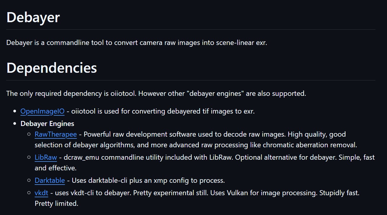
https://github.com/jedypod/debayer
The only required dependency is oiiotool. However other “debayer engines” are also supported.
- OpenImageIO – oiiotool is used for converting debayered tif images to exr.
- Debayer Engines
- RawTherapee – Powerful raw development software used to decode raw images. High quality, good selection of debayer algorithms, and more advanced raw processing like chromatic aberration removal.
- LibRaw – dcraw_emu commandline utility included with LibRaw. Optional alternative for debayer. Simple, fast and effective.
- Darktable – Uses darktable-cli plus an xmp config to process.
- vkdt – uses vkdt-cli to debayer. Pretty experimental still. Uses Vulkan for image processing. Stupidly fast. Pretty limited.
-
HDRI Median Cut plugin
Read more: HDRI Median Cut pluginwww.hdrlabs.com/picturenaut/plugins.html
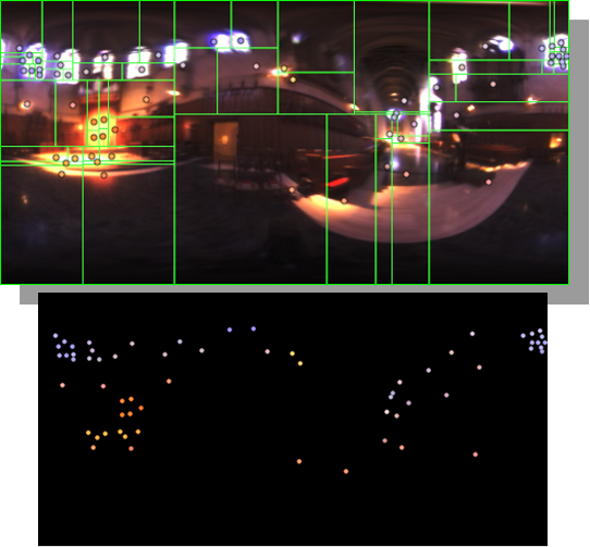
Note. The Median Cut algorithm is typically used for color quantization, which involves reducing the number of colors in an image while preserving its visual quality. It doesn’t directly provide a way to identify the brightest areas in an image. However, if you’re interested in identifying the brightest areas, you might want to look into other methods like thresholding, histogram analysis, or edge detection, through openCV for example.
Here is an openCV example:
# bottom left coordinates = 0,0 import numpy as np import cv2 # Load the HDR or EXR image image = cv2.imread('your_image_path.exr', cv2.IMREAD_UNCHANGED) # Load as-is without modification # Calculate the luminance from the HDR channels (assuming RGB format) luminance = np.dot(image[..., :3], [0.299, 0.587, 0.114]) # Set a threshold value based on estimated EV threshold_value = 2.4 # Estimated threshold value based on 4.8 EV # Apply the threshold to identify bright areas # Theluminancearray contains the calculated luminance values for each pixel in the image. # Thethreshold_valueis a user-defined value that represents a cutoff point, separating "bright" and "dark" areas in terms of perceived luminance.thresholded = (luminance > threshold_value) * 255 # Convert the thresholded image to uint8 for contour detection thresholded = thresholded.astype(np.uint8) # Find contours of the bright areas contours, _ = cv2.findContours(thresholded, cv2.RETR_EXTERNAL, cv2.CHAIN_APPROX_SIMPLE) # Create a list to store the bounding boxes of bright areas bright_areas = [] # Iterate through contours and extract bounding boxes for contour in contours: x, y, w, h = cv2.boundingRect(contour) # Adjust y-coordinate based on bottom-left origin y_bottom_left_origin = image.shape[0] - (y + h) bright_areas.append((x, y_bottom_left_origin, x + w, y_bottom_left_origin + h)) # Store as (x1, y1, x2, y2) # Print the identified bright areas print("Bright Areas (x1, y1, x2, y2):") for area in bright_areas: print(area)More details
Luminance and Exposure in an EXR Image:
- An EXR (Extended Dynamic Range) image format is often used to store high dynamic range (HDR) images that contain a wide range of luminance values, capturing both dark and bright areas.
- Luminance refers to the perceived brightness of a pixel in an image. In an RGB image, luminance is often calculated using a weighted sum of the red, green, and blue channels, where different weights are assigned to each channel to account for human perception.
- In an EXR image, the pixel values can represent radiometrically accurate scene values, including actual radiance or irradiance levels. These values are directly related to the amount of light emitted or reflected by objects in the scene.
The luminance line is calculating the luminance of each pixel in the image using a weighted sum of the red, green, and blue channels. The three float values [0.299, 0.587, 0.114] are the weights used to perform this calculation.
These weights are based on the concept of luminosity, which aims to approximate the perceived brightness of a color by taking into account the human eye’s sensitivity to different colors. The values are often derived from the NTSC (National Television System Committee) standard, which is used in various color image processing operations.
Here’s the breakdown of the float values:
- 0.299: Weight for the red channel.
- 0.587: Weight for the green channel.
- 0.114: Weight for the blue channel.
The weighted sum of these channels helps create a grayscale image where the pixel values represent the perceived brightness. This technique is often used when converting a color image to grayscale or when calculating luminance for certain operations, as it takes into account the human eye’s sensitivity to different colors.
For the threshold, remember that the exact relationship between EV values and pixel values can depend on the tone-mapping or normalization applied to the HDR image, as well as the dynamic range of the image itself.
To establish a relationship between exposure and the threshold value, you can consider the relationship between linear and logarithmic scales:
- Linear and Logarithmic Scales:
- Exposure values in an EXR image are often represented in logarithmic scales, such as EV (exposure value). Each increment in EV represents a doubling or halving of the amount of light captured.
- Threshold values for luminance thresholding are usually linear, representing an actual luminance level.
- Conversion Between Scales:
- To establish a mathematical relationship, you need to convert between the logarithmic exposure scale and the linear threshold scale.
- One common method is to use a power function. For instance, you can use a power function to convert EV to a linear intensity value.
threshold_value = base_value * (2 ** EV)Here,
EVis the exposure value,base_valueis a scaling factor that determines the relationship between EV and threshold_value, and2 ** EVis used to convert the logarithmic EV to a linear intensity value. - Choosing the Base Value:
- The
base_valuefactor should be determined based on the dynamic range of your EXR image and the specific luminance values you are dealing with. - You may need to experiment with different values of
base_valueto achieve the desired separation of bright areas from the rest of the image.
- The
Let’s say you have an EXR image with a dynamic range of 12 EV, which is a common range for many high dynamic range images. In this case, you want to set a threshold value that corresponds to a certain number of EV above the middle gray level (which is often considered to be around 0.18).
Here’s an example of how you might determine a
base_valueto achieve this:# Define the dynamic range of the image in EV dynamic_range = 12 # Choose the desired number of EV above middle gray for thresholding desired_ev_above_middle_gray = 2 # Calculate the threshold value based on the desired EV above middle gray threshold_value = 0.18 * (2 ** (desired_ev_above_middle_gray / dynamic_range)) print("Threshold Value:", threshold_value)
Collections
| Explore posts
| Design And Composition
| Featured AI
Popular Searches
unreal | pipeline | virtual production | free | learn | photoshop | 360 | macro | google | nvidia | resolution | open source | hdri | real-time | photography basics | nuke
FEATURED POSTS
Social Links
DISCLAIMER – Links and images on this website may be protected by the respective owners’ copyright. All data submitted by users through this site shall be treated as freely available to share.




![sRGB gamma correction test [gamma correction test]](http://www.madore.org/~david/misc/color/gammatest.png)

