


COMPOSITION
-
SlowMoVideo – How to make a slow motion shot with the open source program
Read more: SlowMoVideo – How to make a slow motion shot with the open source programhttp://slowmovideo.granjow.net/
slowmoVideo is an OpenSource program that creates slow-motion videos from your footage.
Slow motion cinematography is the result of playing back frames for a longer duration than they were exposed. For example, if you expose 240 frames of film in one second, then play them back at 24 fps, the resulting movie is 10 times longer (slower) than the original filmed event….
Film cameras are relatively simple mechanical devices that allow you to crank up the speed to whatever rate the shutter and pull-down mechanism allow. Some film cameras can operate at 2,500 fps or higher (although film shot in these cameras often needs some readjustment in postproduction). Video, on the other hand, is always captured, recorded, and played back at a fixed rate, with a current limit around 60fps. This makes extreme slow motion effects harder to achieve (and less elegant) on video, because slowing down the video results in each frame held still on the screen for a long time, whereas with high-frame-rate film there are plenty of frames to fill the longer durations of time. On video, the slow motion effect is more like a slide show than smooth, continuous motion.
One obvious solution is to shoot film at high speed, then transfer it to video (a case where film still has a clear advantage, sorry George). Another possibility is to cross dissolve or blur from one frame to the next. This adds a smooth transition from one still frame to the next. The blur reduces the sharpness of the image, and compared to slowing down images shot at a high frame rate, this is somewhat of a cheat. However, there isn’t much you can do about it until video can be recorded at much higher rates. Of course, many film cameras can’t shoot at high frame rates either, so the whole super-slow-motion endeavor is somewhat specialized no matter what medium you are using. (There are some high speed digital cameras available now that allow you to capture lots of digital frames directly to your computer, so technology is starting to catch up with film. However, this feature isn’t going to appear in consumer camcorders any time soon.)


DESIGN
-
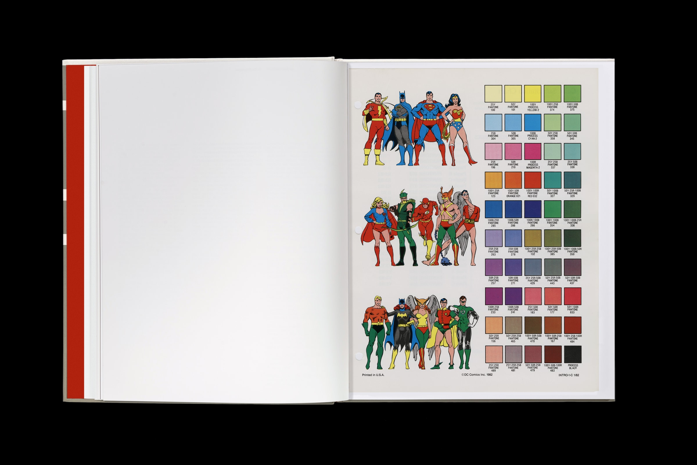
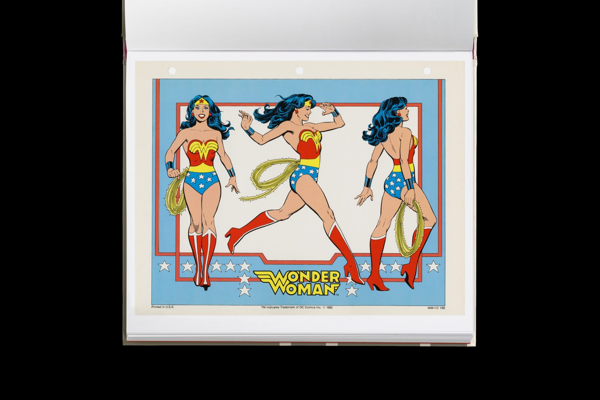
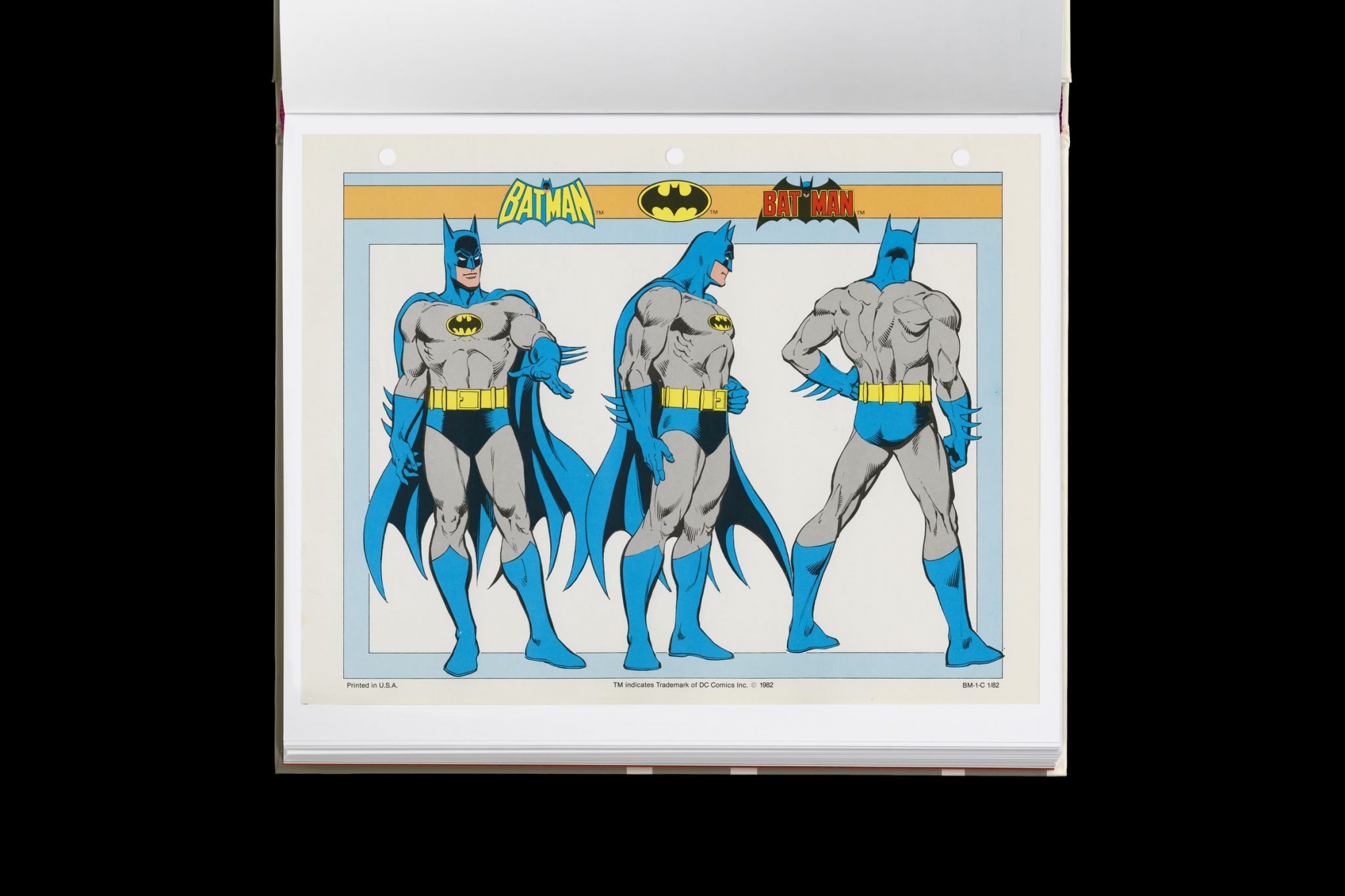
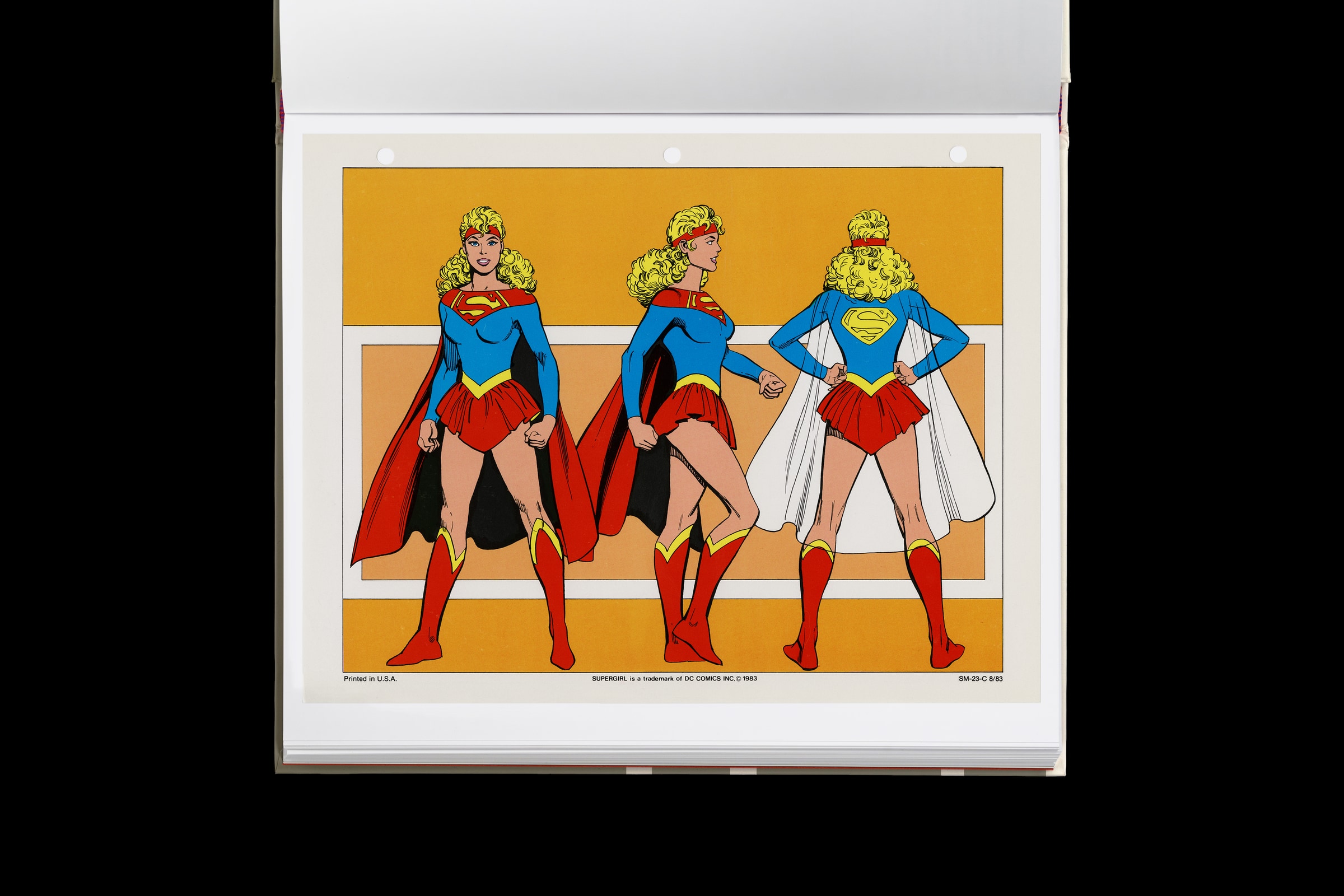
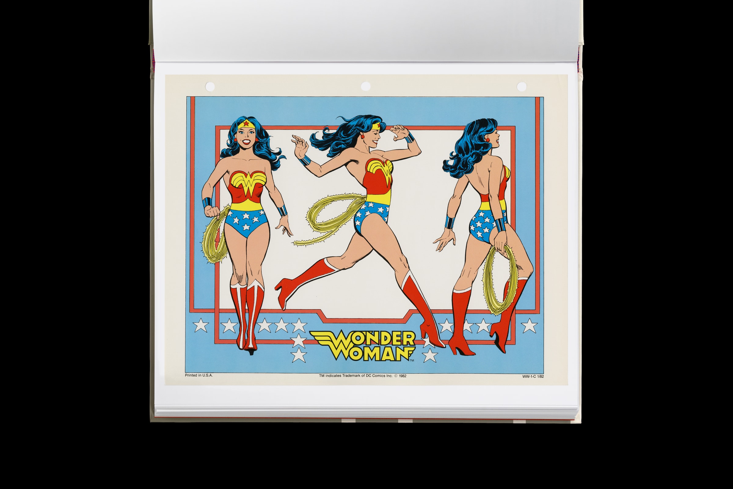
This legendary DC Comics style guide was nearly lost for years – now you can buy it
Read more: This legendary DC Comics style guide was nearly lost for years – now you can buy ithttps://www.fastcompany.com/91133306/dc-comics-style-guide-was-lost-for-years-now-you-can-buy-it
Reproduced from a rare original copy, the book features over 165 highly-detailed scans of the legendary art by José Luis García-López, with an introduction by Paul Levitz, former president of DC Comics.
https://standardsmanual.com/products/1982-dc-comics-style-guide
-
Glenn Marshall – The Crow
Read more: Glenn Marshall – The Crow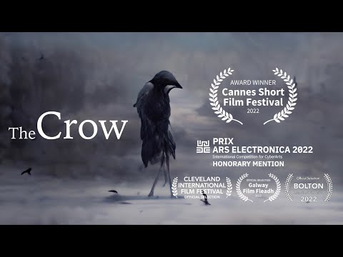
Created with AI ‘Style Transfer’ processes to transform video footage into AI video art.


COLOR
-
Weta Digital – Manuka Raytracer and Gazebo GPU renderers – pipeline
Read more: Weta Digital – Manuka Raytracer and Gazebo GPU renderers – pipelinehttps://jo.dreggn.org/home/2018_manuka.pdf
http://www.fxguide.com/featured/manuka-weta-digitals-new-renderer/

The Manuka rendering architecture has been designed in the spirit of the classic reyes rendering architecture. In its core, reyes is based on stochastic rasterisation of micropolygons, facilitating depth of field, motion blur, high geometric complexity,and programmable shading.
This is commonly achieved with Monte Carlo path tracing, using a paradigm often called shade-on-hit, in which the renderer alternates tracing rays with running shaders on the various ray hits. The shaders take the role of generating the inputs of the local material structure which is then used bypath sampling logic to evaluate contributions and to inform what further rays to cast through the scene.
Over the years, however, the expectations have risen substantially when it comes to image quality. Computing pictures which are indistinguishable from real footage requires accurate simulation of light transport, which is most often performed using some variant of Monte Carlo path tracing. Unfortunately this paradigm requires random memory accesses to the whole scene and does not lend itself well to a rasterisation approach at all.
Manuka is both a uni-directional and bidirectional path tracer and encompasses multiple importance sampling (MIS). Interestingly, and importantly for production character skin work, it is the first major production renderer to incorporate spectral MIS in the form of a new ‘Hero Spectral Sampling’ technique, which was recently published at Eurographics Symposium on Rendering 2014.
Manuka propose a shade-before-hit paradigm in-stead and minimise I/O strain (and some memory costs) on the system, leveraging locality of reference by running pattern generation shaders before we execute light transport simulation by path sampling, “compressing” any bvh structure as needed, and as such also limiting duplication of source data.
The difference with reyes is that instead of baking colors into the geometry like in Reyes, manuka bakes surface closures. This means that light transport is still calculated with path tracing, but all texture lookups etc. are done up-front and baked into the geometry.The main drawback with this method is that geometry has to be tessellated to its highest, stable topology before shading can be evaluated properly. As such, the high cost to first pixel. Even a basic 4 vertices square becomes a much more complex model with this approach.

Manuka use the RenderMan Shading Language (rsl) for programmable shading [Pixar Animation Studios 2015], but we do not invoke rsl shaders when intersecting a ray with a surface (often called shade-on-hit). Instead, we pre-tessellate and pre-shade all the input geometry in the front end of the renderer.
This way, we can efficiently order shading computations to sup-port near-optimal texture locality, vectorisation, and parallelism. This system avoids repeated evaluation of shaders at the same surface point, and presents a minimal amount of memory to be accessed during light transport time. An added benefit is that the acceleration structure for ray tracing (abounding volume hierarchy, bvh) is built once on the final tessellated geometry, which allows us to ray trace more efficiently than multi-level bvhs and avoids costly caching of on-demand tessellated micropolygons and the associated scheduling issues.For the shading reasons above, in terms of AOVs, the studio approach is to succeed at combining complex shading with ray paths in the render rather than pass a multi-pass render to compositing.
For the Spectral Rendering component. The light transport stage is fully spectral, using a continuously sampled wavelength which is traced with each path and used to apply the spectral camera sensitivity of the sensor. This allows for faithfully support any degree of observer metamerism as the camera footage they are intended to match as well as complex materials which require wavelength dependent phenomena such as diffraction, dispersion, interference, iridescence, or chromatic extinction and Rayleigh scattering in participating media.
As opposed to the original reyes paper, we use bilinear interpolation of these bsdf inputs later when evaluating bsdfs per pathv ertex during light transport4. This improves temporal stability of geometry which moves very slowly with respect to the pixel raster
In terms of the pipeline, everything rendered at Weta was already completely interwoven with their deep data pipeline. Manuka very much was written with deep data in mind. Here, Manuka not so much extends the deep capabilities, rather it fully matches the already extremely complex and powerful setup Weta Digital already enjoy with RenderMan. For example, an ape in a scene can be selected, its ID is available and a NUKE artist can then paint in 3D say a hand and part of the way up the neutral posed ape.
We called our system Manuka, as a respectful nod to reyes: we had heard a story froma former ILM employee about how reyes got its name from how fond the early Pixar people were of their lunches at Point Reyes, and decided to name our system after our surrounding natural environment, too. Manuka is a kind of tea tree very common in New Zealand which has very many very small leaves, in analogy to micropolygons ina tree structure for ray tracing. It also happens to be the case that Weta Digital’s main site is on Manuka Street.

-
What is OLED and what can it do for your TV
Read more: What is OLED and what can it do for your TVhttps://www.cnet.com/news/what-is-oled-and-what-can-it-do-for-your-tv/
OLED stands for Organic Light Emitting Diode. Each pixel in an OLED display is made of a material that glows when you jab it with electricity. Kind of like the heating elements in a toaster, but with less heat and better resolution. This effect is called electroluminescence, which is one of those delightful words that is big, but actually makes sense: “electro” for electricity, “lumin” for light and “escence” for, well, basically “essence.”
OLED TV marketing often claims “infinite” contrast ratios, and while that might sound like typical hyperbole, it’s one of the extremely rare instances where such claims are actually true. Since OLED can produce a perfect black, emitting no light whatsoever, its contrast ratio (expressed as the brightest white divided by the darkest black) is technically infinite.
OLED is the only technology capable of absolute blacks and extremely bright whites on a per-pixel basis. LCD definitely can’t do that, and even the vaunted, beloved, dearly departed plasma couldn’t do absolute blacks.
-
HDR and Color
Read more: HDR and Colorhttps://www.soundandvision.com/content/nits-and-bits-hdr-and-color
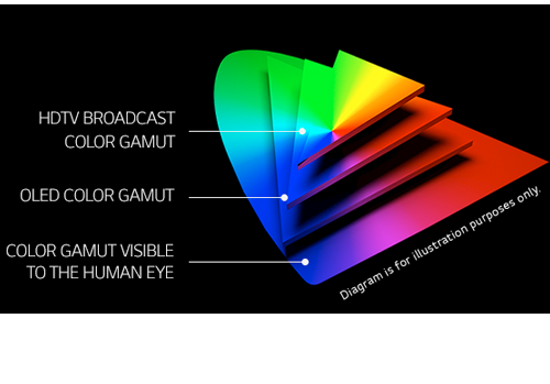
In HD we often refer to the range of available colors as a color gamut. Such a color gamut is typically plotted on a two-dimensional diagram, called a CIE chart, as shown in at the top of this blog. Each color is characterized by its x/y coordinates.

Good enough for government work, perhaps. But for HDR, with its higher luminance levels and wider color, the gamut becomes three-dimensional.

For HDR the color gamut therefore becomes a characteristic we now call the color volume. It isn’t easy to show color volume on a two-dimensional medium like the printed page or a computer screen, but one method is shown below. As the luminance becomes higher, the picture eventually turns to white. As it becomes darker, it fades to black. The traditional color gamut shown on the CIE chart is simply a slice through this color volume at a selected luminance level, such as 50%.
Three different color volumes—we still refer to them as color gamuts though their third dimension is important—are currently the most significant. The first is BT.709 (sometimes referred to as Rec.709), the color gamut used for pre-UHD/HDR formats, including standard HD.
The largest is known as BT.2020; it encompasses (roughly) the range of colors visible to the human eye (though ET might find it insufficient!).
Between these two is the color gamut used in digital cinema, known as DCI-P3.

sRGB

D65

-
VES Cinematic Color – Motion-Picture Color Management
Read more: VES Cinematic Color – Motion-Picture Color ManagementThis paper presents an introduction to the color pipelines behind modern feature-film visual-effects and animation.
Authored by Jeremy Selan, and reviewed by the members of the VES Technology Committee including Rob Bredow, Dan Candela, Nick Cannon, Paul Debevec, Ray Feeney, Andy Hendrickson, Gautham Krishnamurti, Sam Richards, Jordan Soles, and Sebastian Sylwan.
-
PBR Color Reference List for Materials – by Grzegorz Baran
Read more: PBR Color Reference List for Materials – by Grzegorz Baran
“The list should be helpful for every material artist who work on PBR materials as it contains over 200 color values measured with PCE-RGB2 1002 Color Spectrometer device and presented in linear and sRGB (2.2) gamma space.
All color values, HUE and Saturation in this list come from measurements taken with PCE-RGB2 1002 Color Spectrometer device and are presented in linear and sRGB (2.2) gamma space (more info at the end of this video) I calculated Relative Luminance and Luminance values based on captured color using my own equation which takes color based luminance perception into consideration. Bare in mind that there is no ‘one’ color per substance as nothing in nature is even 100% uniform and any value in +/-10% range from these should be considered as correct one. Therefore this list should be always considered as a color reference for material’s albedos, not ulitimate and absolute truth.“
-
What is a Gamut or Color Space and why do I need to know about CIE
Read more: What is a Gamut or Color Space and why do I need to know about CIE

http://www.xdcam-user.com/2014/05/what-is-a-gamut-or-color-space-and-why-do-i-need-to-know-about-it/
In video terms gamut is normally related to as the full range of colours and brightness that can be either captured or displayed.
Generally speaking all color gamuts recommendations are trying to define a reasonable level of color representation based on available technology and hardware. REC-601 represents the old TVs. REC-709 is currently the most distributed solution. P3 is mainly available in movie theaters and is now being adopted in some of the best new 4K HDR TVs. Rec2020 (a wider space than P3 that improves on visibke color representation) and ACES (the full coverage of visible color) are other common standards which see major hardware development these days.

To compare and visualize different solution (across video and printing solutions), most developers use the CIE color model chart as a reference.
The CIE color model is a color space model created by the International Commission on Illumination known as the Commission Internationale de l’Elcairage (CIE) in 1931. It is also known as the CIE XYZ color space or the CIE 1931 XYZ color space.
This chart represents the first defined quantitative link between distributions of wavelengths in the electromagnetic visible spectrum, and physiologically perceived colors in human color vision. Or basically, the range of color a typical human eye can perceive through visible light.
Note that while the human perception is quite wide, and generally speaking biased towards greens (we are apes after all), the amount of colors available through nature, generated through light reflection, tend to be a much smaller section. This is defined by the Pointer’s Chart.


In short. Color gamut is a representation of color coverage, used to describe data stored in images against available hardware and viewer technologies.
Camera color encoding from
https://www.slideshare.net/hpduiker/acescg-a-common-color-encoding-for-visual-effects-applications
CIE 1976
http://bernardsmith.eu/computatrum/scan_and_restore_archive_and_print/scanning/
https://store.yujiintl.com/blogs/high-cri-led/understanding-cie1931-and-cie-1976
The CIE 1931 standard has been replaced by a CIE 1976 standard. Below we can see the significance of this.
People have observed that the biggest issue with CIE 1931 is the lack of uniformity with chromaticity, the three dimension color space in rectangular coordinates is not visually uniformed.
The CIE 1976 (also called CIELUV) was created by the CIE in 1976. It was put forward in an attempt to provide a more uniform color spacing than CIE 1931 for colors at approximately the same luminance
The CIE 1976 standard colour space is more linear and variations in perceived colour between different people has also been reduced. The disproportionately large green-turquoise area in CIE 1931, which cannot be generated with existing computer screens, has been reduced.
If we move from CIE 1931 to the CIE 1976 standard colour space we can see that the improvements made in the gamut for the “new” iPad screen (as compared to the “old” iPad 2) are more evident in the CIE 1976 colour space than in the CIE 1931 colour space, particularly in the blues from aqua to deep blue.

https://dot-color.com/2012/08/14/color-space-confusion/
Despite its age, CIE 1931, named for the year of its adoption, remains a well-worn and familiar shorthand throughout the display industry. CIE 1931 is the primary language of customers. When a customer says that their current display “can do 72% of NTSC,” they implicitly mean 72% of NTSC 1953 color gamut as mapped against CIE 1931.
-
Willem Zwarthoed – Aces gamut in VFX production pdf
Read more: Willem Zwarthoed – Aces gamut in VFX production pdfhttps://www.provideocoalition.com/color-management-part-12-introducing-aces/
Local copy:
https://www.slideshare.net/hpduiker/acescg-a-common-color-encoding-for-visual-effects-applications
-
OpenColorIO standard
Read more: OpenColorIO standardhttps://www.provideocoalition.com/color-management-part-11-introducing-opencolorio/
OpenColorIO (OCIO) is a new open source project from Sony Imageworks.
Based on development started in 2003, OCIO enables color transforms and image display to be handled in a consistent manner across multiple graphics applications. Unlike other color management solutions, OCIO is geared towards motion-picture post production, with an emphasis on visual effects and animation color pipelines.


LIGHTING
-
Key/Fill ratios and scene composition using false colors
Read more: Key/Fill ratios and scene composition using false colors
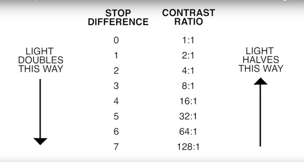
To measure the contrast ratio you will need a light meter. The process starts with you measuring the main source of light, or the key light.
Get a reading from the brightest area on the face of your subject. Then, measure the area lit by the secondary light, or fill light. To make sense of what you have just measured you have to understand that the information you have just gathered is in F-stops, a measure of light. With each additional F-stop, for example going one stop from f/1.4 to f/2.0, you create a doubling of light. The reverse is also true; moving one stop from f/8.0 to f/5.6 results in a halving of the light.
Let’s say you grabbed a measurement from your key light of f/8.0. Then, when you measured your fill light area, you get a reading of f/4.0. This will lead you to a contrast ratio of 4:1 because there are two stops between f/4.0 and f/8.0 and each stop doubles the amount of light. In other words, two stops x twice the light per stop = four times as much light at f/8.0 than at f/4.0.

theslantedlens.com/2017/lighting-ratios-photo-video/
Examples in the post
-
3D Lighting Tutorial by Amaan Kram
Read more: 3D Lighting Tutorial by Amaan Kramhttp://www.amaanakram.com/lightingT/part1.htm
The goals of lighting in 3D computer graphics are more or less the same as those of real world lighting.
Lighting serves a basic function of bringing out, or pushing back the shapes of objects visible from the camera’s view.
It gives a two-dimensional image on the monitor an illusion of the third dimension-depth.But it does not just stop there. It gives an image its personality, its character. A scene lit in different ways can give a feeling of happiness, of sorrow, of fear etc., and it can do so in dramatic or subtle ways. Along with personality and character, lighting fills a scene with emotion that is directly transmitted to the viewer.
Trying to simulate a real environment in an artificial one can be a daunting task. But even if you make your 3D rendering look absolutely photo-realistic, it doesn’t guarantee that the image carries enough emotion to elicit a “wow” from the people viewing it.
Making 3D renderings photo-realistic can be hard. Putting deep emotions in them can be even harder. However, if you plan out your lighting strategy for the mood and emotion that you want your rendering to express, you make the process easier for yourself.
Each light source can be broken down in to 4 distinct components and analyzed accordingly.
· Intensity
· Direction
· Color
· SizeThe overall thrust of this writing is to produce photo-realistic images by applying good lighting techniques.

-
Photography basics: Lumens vs Candelas (candle) vs Lux vs FootCandle vs Watts vs Irradiance vs Illuminance
Read more: Photography basics: Lumens vs Candelas (candle) vs Lux vs FootCandle vs Watts vs Irradiance vs Illuminancehttps://www.translatorscafe.com/unit-converter/en-US/illumination/1-11/

The power output of a light source is measured using the unit of watts W. This is a direct measure to calculate how much power the light is going to drain from your socket and it is not relatable to the light brightness itself.
The amount of energy emitted from it per second. That energy comes out in a form of photons which we can crudely represent with rays of light coming out of the source. The higher the power the more rays emitted from the source in a unit of time.
Not all energy emitted is visible to the human eye, so we often rely on photometric measurements, which takes in account the sensitivity of human eye to different wavelenghts


Details in the post
(more…) -
HDRI Median Cut plugin
Read more: HDRI Median Cut pluginwww.hdrlabs.com/picturenaut/plugins.html

Note. The Median Cut algorithm is typically used for color quantization, which involves reducing the number of colors in an image while preserving its visual quality. It doesn’t directly provide a way to identify the brightest areas in an image. However, if you’re interested in identifying the brightest areas, you might want to look into other methods like thresholding, histogram analysis, or edge detection, through openCV for example.
Here is an openCV example:
# bottom left coordinates = 0,0 import numpy as np import cv2 # Load the HDR or EXR image image = cv2.imread('your_image_path.exr', cv2.IMREAD_UNCHANGED) # Load as-is without modification # Calculate the luminance from the HDR channels (assuming RGB format) luminance = np.dot(image[..., :3], [0.299, 0.587, 0.114]) # Set a threshold value based on estimated EV threshold_value = 2.4 # Estimated threshold value based on 4.8 EV # Apply the threshold to identify bright areas # Theluminancearray contains the calculated luminance values for each pixel in the image. # Thethreshold_valueis a user-defined value that represents a cutoff point, separating "bright" and "dark" areas in terms of perceived luminance.thresholded = (luminance > threshold_value) * 255 # Convert the thresholded image to uint8 for contour detection thresholded = thresholded.astype(np.uint8) # Find contours of the bright areas contours, _ = cv2.findContours(thresholded, cv2.RETR_EXTERNAL, cv2.CHAIN_APPROX_SIMPLE) # Create a list to store the bounding boxes of bright areas bright_areas = [] # Iterate through contours and extract bounding boxes for contour in contours: x, y, w, h = cv2.boundingRect(contour) # Adjust y-coordinate based on bottom-left origin y_bottom_left_origin = image.shape[0] - (y + h) bright_areas.append((x, y_bottom_left_origin, x + w, y_bottom_left_origin + h)) # Store as (x1, y1, x2, y2) # Print the identified bright areas print("Bright Areas (x1, y1, x2, y2):") for area in bright_areas: print(area)More details
Luminance and Exposure in an EXR Image:
- An EXR (Extended Dynamic Range) image format is often used to store high dynamic range (HDR) images that contain a wide range of luminance values, capturing both dark and bright areas.
- Luminance refers to the perceived brightness of a pixel in an image. In an RGB image, luminance is often calculated using a weighted sum of the red, green, and blue channels, where different weights are assigned to each channel to account for human perception.
- In an EXR image, the pixel values can represent radiometrically accurate scene values, including actual radiance or irradiance levels. These values are directly related to the amount of light emitted or reflected by objects in the scene.
The luminance line is calculating the luminance of each pixel in the image using a weighted sum of the red, green, and blue channels. The three float values [0.299, 0.587, 0.114] are the weights used to perform this calculation.
These weights are based on the concept of luminosity, which aims to approximate the perceived brightness of a color by taking into account the human eye’s sensitivity to different colors. The values are often derived from the NTSC (National Television System Committee) standard, which is used in various color image processing operations.
Here’s the breakdown of the float values:
- 0.299: Weight for the red channel.
- 0.587: Weight for the green channel.
- 0.114: Weight for the blue channel.
The weighted sum of these channels helps create a grayscale image where the pixel values represent the perceived brightness. This technique is often used when converting a color image to grayscale or when calculating luminance for certain operations, as it takes into account the human eye’s sensitivity to different colors.
For the threshold, remember that the exact relationship between EV values and pixel values can depend on the tone-mapping or normalization applied to the HDR image, as well as the dynamic range of the image itself.
To establish a relationship between exposure and the threshold value, you can consider the relationship between linear and logarithmic scales:
- Linear and Logarithmic Scales:
- Exposure values in an EXR image are often represented in logarithmic scales, such as EV (exposure value). Each increment in EV represents a doubling or halving of the amount of light captured.
- Threshold values for luminance thresholding are usually linear, representing an actual luminance level.
- Conversion Between Scales:
- To establish a mathematical relationship, you need to convert between the logarithmic exposure scale and the linear threshold scale.
- One common method is to use a power function. For instance, you can use a power function to convert EV to a linear intensity value.
threshold_value = base_value * (2 ** EV)Here,
EVis the exposure value,base_valueis a scaling factor that determines the relationship between EV and threshold_value, and2 ** EVis used to convert the logarithmic EV to a linear intensity value. - Choosing the Base Value:
- The
base_valuefactor should be determined based on the dynamic range of your EXR image and the specific luminance values you are dealing with. - You may need to experiment with different values of
base_valueto achieve the desired separation of bright areas from the rest of the image.
- The
Let’s say you have an EXR image with a dynamic range of 12 EV, which is a common range for many high dynamic range images. In this case, you want to set a threshold value that corresponds to a certain number of EV above the middle gray level (which is often considered to be around 0.18).
Here’s an example of how you might determine a
base_valueto achieve this:# Define the dynamic range of the image in EV dynamic_range = 12 # Choose the desired number of EV above middle gray for thresholding desired_ev_above_middle_gray = 2 # Calculate the threshold value based on the desired EV above middle gray threshold_value = 0.18 * (2 ** (desired_ev_above_middle_gray / dynamic_range)) print("Threshold Value:", threshold_value)


COLLECTIONS
| Featured AI
| Design And Composition
| Explore posts
POPULAR SEARCHES
unreal | pipeline | virtual production | free | learn | photoshop | 360 | macro | google | nvidia | resolution | open source | hdri | real-time | photography basics | nuke
FEATURED POSTS
-
QR code logos
-
VFX pipeline – Render Wall management topics
-
PixelSham – Introduction to Python 2022
-
Methods for creating motion blur in Stop motion
-
Free fonts
-
Google – Artificial Intelligence free courses
-
Photography basics: Color Temperature and White Balance
-
Ross Pettit on The Agile Manager – How tech firms went for prioritizing cash flow instead of talent
Social Links
DISCLAIMER – Links and images on this website may be protected by the respective owners’ copyright. All data submitted by users through this site shall be treated as freely available to share.
