COMPOSITION
-
9 Best Hacks to Make a Cinematic Video with Any Camera
Read more: 9 Best Hacks to Make a Cinematic Video with Any Camerahttps://www.flexclip.com/learn/cinematic-video.html
- Frame Your Shots to Create Depth
- Create Shallow Depth of Field
- Avoid Shaky Footage and Use Flexible Camera Movements
- Properly Use Slow Motion
- Use Cinematic Lighting Techniques
- Apply Color Grading
- Use Cinematic Music and SFX
- Add Cinematic Fonts and Text Effects
- Create the Cinematic Bar at the Top and the Bottom
DESIGN
COLOR
-
Björn Ottosson – OKHSV and OKHSL – Two new color spaces for color picking
Read more: Björn Ottosson – OKHSV and OKHSL – Two new color spaces for color pickinghttps://bottosson.github.io/misc/colorpicker
https://bottosson.github.io/posts/colorpicker/
https://www.smashingmagazine.com/2024/10/interview-bjorn-ottosson-creator-oklab-color-space/
One problem with sRGB is that in a gradient between blue and white, it becomes a bit purple in the middle of the transition. That’s because sRGB really isn’t created to mimic how the eye sees colors; rather, it is based on how CRT monitors work. That means it works with certain frequencies of red, green, and blue, and also the non-linear coding called gamma. It’s a miracle it works as well as it does, but it’s not connected to color perception. When using those tools, you sometimes get surprising results, like purple in the gradient.
There were also attempts to create simple models matching human perception based on XYZ, but as it turned out, it’s not possible to model all color vision that way. Perception of color is incredibly complex and depends, among other things, on whether it is dark or light in the room and the background color it is against. When you look at a photograph, it also depends on what you think the color of the light source is. The dress is a typical example of color vision being very context-dependent. It is almost impossible to model this perfectly.
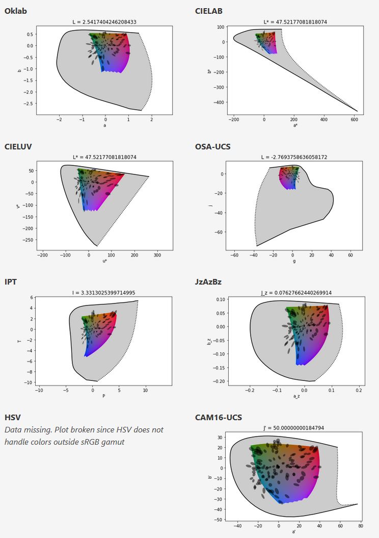
I based Oklab on two other color spaces, CIECAM16 and IPT. I used the lightness and saturation prediction from CIECAM16, which is a color appearance model, as a target. I actually wanted to use the datasets used to create CIECAM16, but I couldn’t find them.
IPT was designed to have better hue uniformity. In experiments, they asked people to match light and dark colors, saturated and unsaturated colors, which resulted in a dataset for which colors, subjectively, have the same hue. IPT has a few other issues but is the basis for hue in Oklab.
In the Munsell color system, colors are described with three parameters, designed to match the perceived appearance of colors: Hue, Chroma and Value. The parameters are designed to be independent and each have a uniform scale. This results in a color solid with an irregular shape. The parameters are designed to be independent and each have a uniform scale. This results in a color solid with an irregular shape. Modern color spaces and models, such as CIELAB, Cam16 and Björn Ottosson own Oklab, are very similar in their construction.
By far the most used color spaces today for color picking are HSL and HSV, two representations introduced in the classic 1978 paper “Color Spaces for Computer Graphics”. HSL and HSV designed to roughly correlate with perceptual color properties while being very simple and cheap to compute.
Today HSL and HSV are most commonly used together with the sRGB color space.
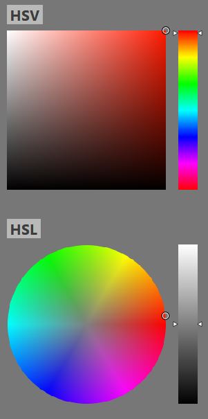
One of the main advantages of HSL and HSV over the different Lab color spaces is that they map the sRGB gamut to a cylinder. This makes them easy to use since all parameters can be changed independently, without the risk of creating colors outside of the target gamut.
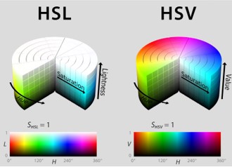
The main drawback on the other hand is that their properties don’t match human perception particularly well.
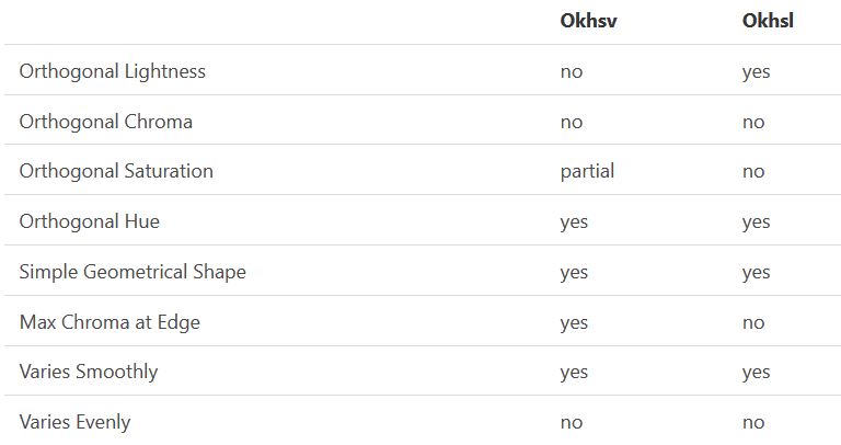
Reconciling these conflicting goals perfectly isn’t possible, but given that HSV and HSL don’t use anything derived from experiments relating to human perception, creating something that makes a better tradeoff does not seem unreasonable.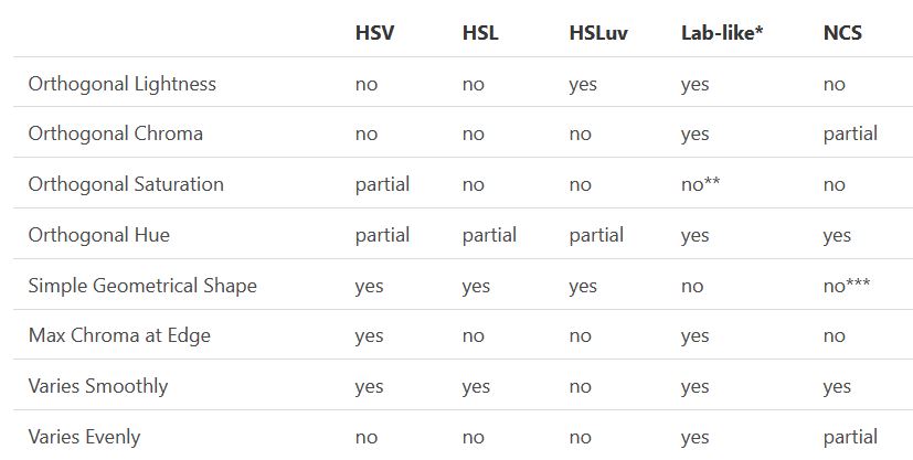
With this new lightness estimate, we are ready to look into the construction of Okhsv and Okhsl.
LIGHTING
-
HDRI Median Cut plugin
Read more: HDRI Median Cut pluginwww.hdrlabs.com/picturenaut/plugins.html
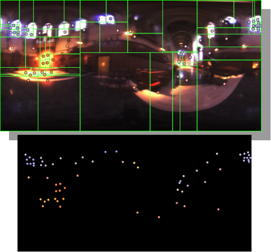
Note. The Median Cut algorithm is typically used for color quantization, which involves reducing the number of colors in an image while preserving its visual quality. It doesn’t directly provide a way to identify the brightest areas in an image. However, if you’re interested in identifying the brightest areas, you might want to look into other methods like thresholding, histogram analysis, or edge detection, through openCV for example.
Here is an openCV example:
# bottom left coordinates = 0,0 import numpy as np import cv2 # Load the HDR or EXR image image = cv2.imread('your_image_path.exr', cv2.IMREAD_UNCHANGED) # Load as-is without modification # Calculate the luminance from the HDR channels (assuming RGB format) luminance = np.dot(image[..., :3], [0.299, 0.587, 0.114]) # Set a threshold value based on estimated EV threshold_value = 2.4 # Estimated threshold value based on 4.8 EV # Apply the threshold to identify bright areas # Theluminancearray contains the calculated luminance values for each pixel in the image. # Thethreshold_valueis a user-defined value that represents a cutoff point, separating "bright" and "dark" areas in terms of perceived luminance.thresholded = (luminance > threshold_value) * 255 # Convert the thresholded image to uint8 for contour detection thresholded = thresholded.astype(np.uint8) # Find contours of the bright areas contours, _ = cv2.findContours(thresholded, cv2.RETR_EXTERNAL, cv2.CHAIN_APPROX_SIMPLE) # Create a list to store the bounding boxes of bright areas bright_areas = [] # Iterate through contours and extract bounding boxes for contour in contours: x, y, w, h = cv2.boundingRect(contour) # Adjust y-coordinate based on bottom-left origin y_bottom_left_origin = image.shape[0] - (y + h) bright_areas.append((x, y_bottom_left_origin, x + w, y_bottom_left_origin + h)) # Store as (x1, y1, x2, y2) # Print the identified bright areas print("Bright Areas (x1, y1, x2, y2):") for area in bright_areas: print(area)More details
Luminance and Exposure in an EXR Image:
- An EXR (Extended Dynamic Range) image format is often used to store high dynamic range (HDR) images that contain a wide range of luminance values, capturing both dark and bright areas.
- Luminance refers to the perceived brightness of a pixel in an image. In an RGB image, luminance is often calculated using a weighted sum of the red, green, and blue channels, where different weights are assigned to each channel to account for human perception.
- In an EXR image, the pixel values can represent radiometrically accurate scene values, including actual radiance or irradiance levels. These values are directly related to the amount of light emitted or reflected by objects in the scene.
The luminance line is calculating the luminance of each pixel in the image using a weighted sum of the red, green, and blue channels. The three float values [0.299, 0.587, 0.114] are the weights used to perform this calculation.
These weights are based on the concept of luminosity, which aims to approximate the perceived brightness of a color by taking into account the human eye’s sensitivity to different colors. The values are often derived from the NTSC (National Television System Committee) standard, which is used in various color image processing operations.
Here’s the breakdown of the float values:
- 0.299: Weight for the red channel.
- 0.587: Weight for the green channel.
- 0.114: Weight for the blue channel.
The weighted sum of these channels helps create a grayscale image where the pixel values represent the perceived brightness. This technique is often used when converting a color image to grayscale or when calculating luminance for certain operations, as it takes into account the human eye’s sensitivity to different colors.
For the threshold, remember that the exact relationship between EV values and pixel values can depend on the tone-mapping or normalization applied to the HDR image, as well as the dynamic range of the image itself.
To establish a relationship between exposure and the threshold value, you can consider the relationship between linear and logarithmic scales:
- Linear and Logarithmic Scales:
- Exposure values in an EXR image are often represented in logarithmic scales, such as EV (exposure value). Each increment in EV represents a doubling or halving of the amount of light captured.
- Threshold values for luminance thresholding are usually linear, representing an actual luminance level.
- Conversion Between Scales:
- To establish a mathematical relationship, you need to convert between the logarithmic exposure scale and the linear threshold scale.
- One common method is to use a power function. For instance, you can use a power function to convert EV to a linear intensity value.
threshold_value = base_value * (2 ** EV)Here,
EVis the exposure value,base_valueis a scaling factor that determines the relationship between EV and threshold_value, and2 ** EVis used to convert the logarithmic EV to a linear intensity value. - Choosing the Base Value:
- The
base_valuefactor should be determined based on the dynamic range of your EXR image and the specific luminance values you are dealing with. - You may need to experiment with different values of
base_valueto achieve the desired separation of bright areas from the rest of the image.
- The
Let’s say you have an EXR image with a dynamic range of 12 EV, which is a common range for many high dynamic range images. In this case, you want to set a threshold value that corresponds to a certain number of EV above the middle gray level (which is often considered to be around 0.18).
Here’s an example of how you might determine a
base_valueto achieve this:# Define the dynamic range of the image in EV dynamic_range = 12 # Choose the desired number of EV above middle gray for thresholding desired_ev_above_middle_gray = 2 # Calculate the threshold value based on the desired EV above middle gray threshold_value = 0.18 * (2 ** (desired_ev_above_middle_gray / dynamic_range)) print("Threshold Value:", threshold_value) -
Fast, optimized ‘for’ pixel loops with OpenCV and Python to create tone mapped HDR images
Read more: Fast, optimized ‘for’ pixel loops with OpenCV and Python to create tone mapped HDR imageshttps://pyimagesearch.com/2017/08/28/fast-optimized-for-pixel-loops-with-opencv-and-python/
https://learnopencv.com/exposure-fusion-using-opencv-cpp-python/
Exposure Fusion is a method for combining images taken with different exposure settings into one image that looks like a tone mapped High Dynamic Range (HDR) image.
Collections
| Explore posts
| Design And Composition
| Featured AI
Popular Searches
unreal | pipeline | virtual production | free | learn | photoshop | 360 | macro | google | nvidia | resolution | open source | hdri | real-time | photography basics | nuke
FEATURED POSTS
Social Links
DISCLAIMER – Links and images on this website may be protected by the respective owners’ copyright. All data submitted by users through this site shall be treated as freely available to share.


