


COMPOSITION
DESIGN
COLOR
-
Yasuharu YOSHIZAWA – Comparison of sRGB vs ACREScg in Nuke
Read more: Yasuharu YOSHIZAWA – Comparison of sRGB vs ACREScg in NukeAnswering the question that is often asked, “Do I need to use ACEScg to display an sRGB monitor in the end?” (Demonstration shown at an in-house seminar)
Comparison of scanlineRender output with extreme color lights on color charts with sRGB/ACREScg in color – OCIO -working space in NukeDownload the Nuke script:
-
VES Cinematic Color – Motion-Picture Color Management
Read more: VES Cinematic Color – Motion-Picture Color ManagementThis paper presents an introduction to the color pipelines behind modern feature-film visual-effects and animation.
Authored by Jeremy Selan, and reviewed by the members of the VES Technology Committee including Rob Bredow, Dan Candela, Nick Cannon, Paul Debevec, Ray Feeney, Andy Hendrickson, Gautham Krishnamurti, Sam Richards, Jordan Soles, and Sebastian Sylwan.
-
Björn Ottosson – How software gets color wrong
Read more: Björn Ottosson – How software gets color wronghttps://bottosson.github.io/posts/colorwrong/
Most software around us today are decent at accurately displaying colors. Processing of colors is another story unfortunately, and is often done badly.
To understand what the problem is, let’s start with an example of three ways of blending green and magenta:
- Perceptual blend – A smooth transition using a model designed to mimic human perception of color. The blending is done so that the perceived brightness and color varies smoothly and evenly.
- Linear blend – A model for blending color based on how light behaves physically. This type of blending can occur in many ways naturally, for example when colors are blended together by focus blur in a camera or when viewing a pattern of two colors at a distance.
- sRGB blend – This is how colors would normally be blended in computer software, using sRGB to represent the colors.

Let’s look at some more examples of blending of colors, to see how these problems surface more practically. The examples use strong colors since then the differences are more pronounced. This is using the same three ways of blending colors as the first example.

Instead of making it as easy as possible to work with color, most software make it unnecessarily hard, by doing image processing with representations not designed for it. Approximating the physical behavior of light with linear RGB models is one easy thing to do, but more work is needed to create image representations tailored for image processing and human perception.
Also see:


![[gamma correction test]](http://www.madore.org/~david/misc/color/gammatest.png "sRGB gamma correction test")


LIGHTING
-
Rec-2020 – TVs new color gamut standard used by Dolby Vision?
Read more: Rec-2020 – TVs new color gamut standard used by Dolby Vision?https://www.hdrsoft.com/resources/dri.html#bit-depth

The dynamic range is a ratio between the maximum and minimum values of a physical measurement. Its definition depends on what the dynamic range refers to.
For a scene: Dynamic range is the ratio between the brightest and darkest parts of the scene.
For a camera: Dynamic range is the ratio of saturation to noise. More specifically, the ratio of the intensity that just saturates the camera to the intensity that just lifts the camera response one standard deviation above camera noise.
For a display: Dynamic range is the ratio between the maximum and minimum intensities emitted from the screen.
The Dynamic Range of real-world scenes can be quite high — ratios of 100,000:1 are common in the natural world. An HDR (High Dynamic Range) image stores pixel values that span the whole tonal range of real-world scenes. Therefore, an HDR image is encoded in a format that allows the largest range of values, e.g. floating-point values stored with 32 bits per color channel. Another characteristics of an HDR image is that it stores linear values. This means that the value of a pixel from an HDR image is proportional to the amount of light measured by the camera.
For TVs HDR is great, but it’s not the only new TV feature worth discussing.
(more…) -
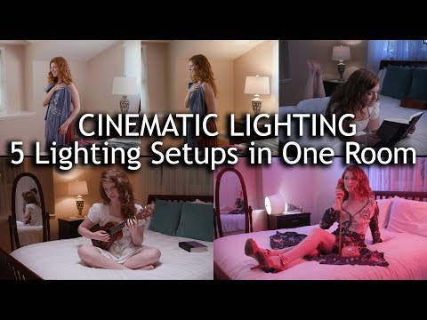
studiobinder.com – What is Tenebrism and Hard Lighting — The Art of Light and Shadow and chiaroscuro Explained
Read more: studiobinder.com – What is Tenebrism and Hard Lighting — The Art of Light and Shadow and chiaroscuro Explainedhttps://www.studiobinder.com/blog/what-is-tenebrism-art-definition/
https://www.studiobinder.com/blog/what-is-hard-light-photography/


-
Composition – cinematography Cheat Sheet
Read more: Composition – cinematography Cheat Sheet
Where is our eye attracted first? Why?
Size. Focus. Lighting. Color.
Size. Mr. White (Harvey Keitel) on the right.
Focus. He’s one of the two objects in focus.
Lighting. Mr. White is large and in focus and Mr. Pink (Steve Buscemi) is highlighted by
a shaft of light.
Color. Both are black and white but the read on Mr. White’s shirt now really stands out.
(more…)
What type of lighting?


COLLECTIONS
| Featured AI
| Design And Composition
| Explore posts
POPULAR SEARCHES
unreal | pipeline | virtual production | free | learn | photoshop | 360 | macro | google | nvidia | resolution | open source | hdri | real-time | photography basics | nuke
FEATURED POSTS
Social Links
DISCLAIMER – Links and images on this website may be protected by the respective owners’ copyright. All data submitted by users through this site shall be treated as freely available to share.
