


COMPOSITION
-
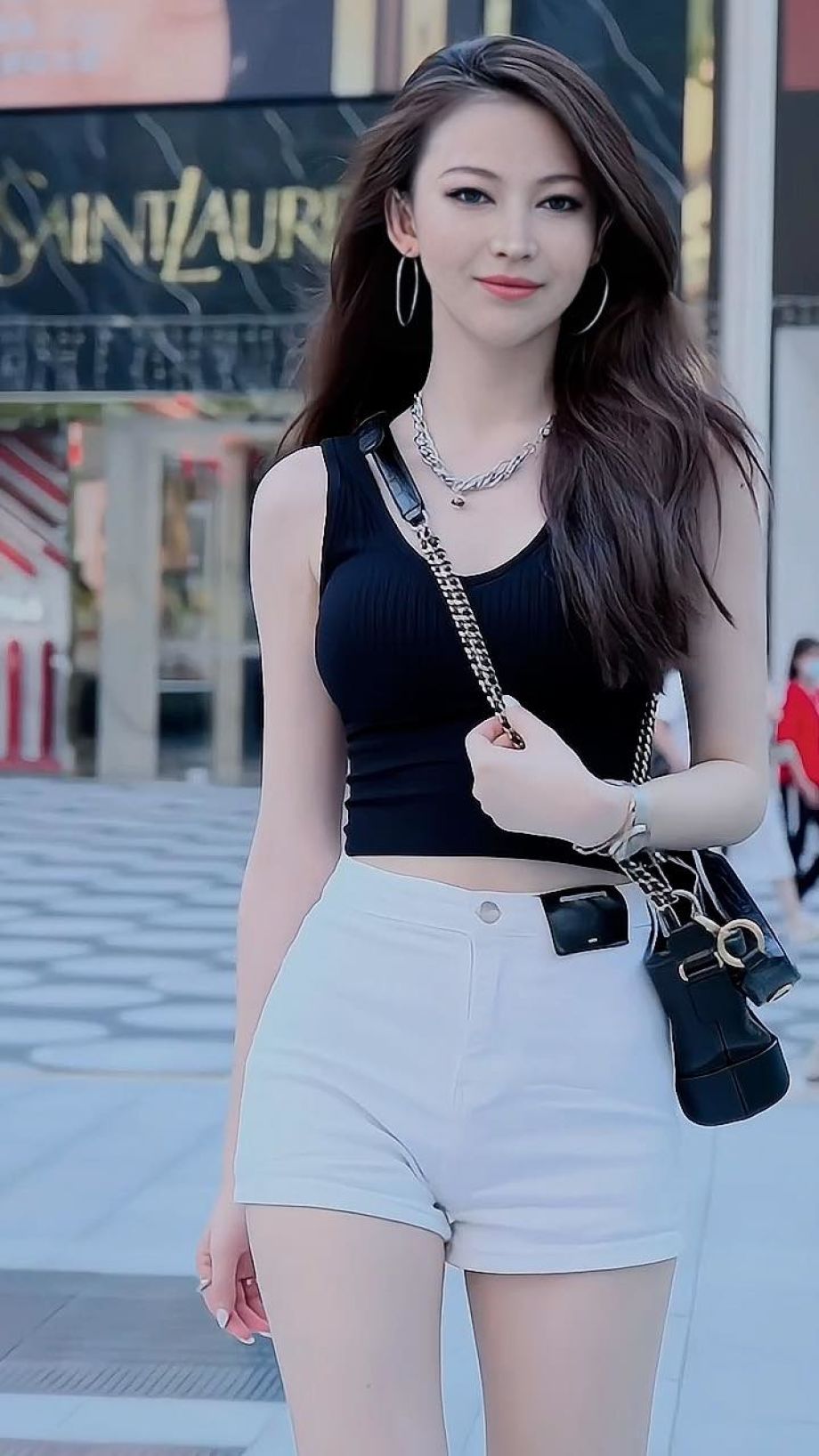
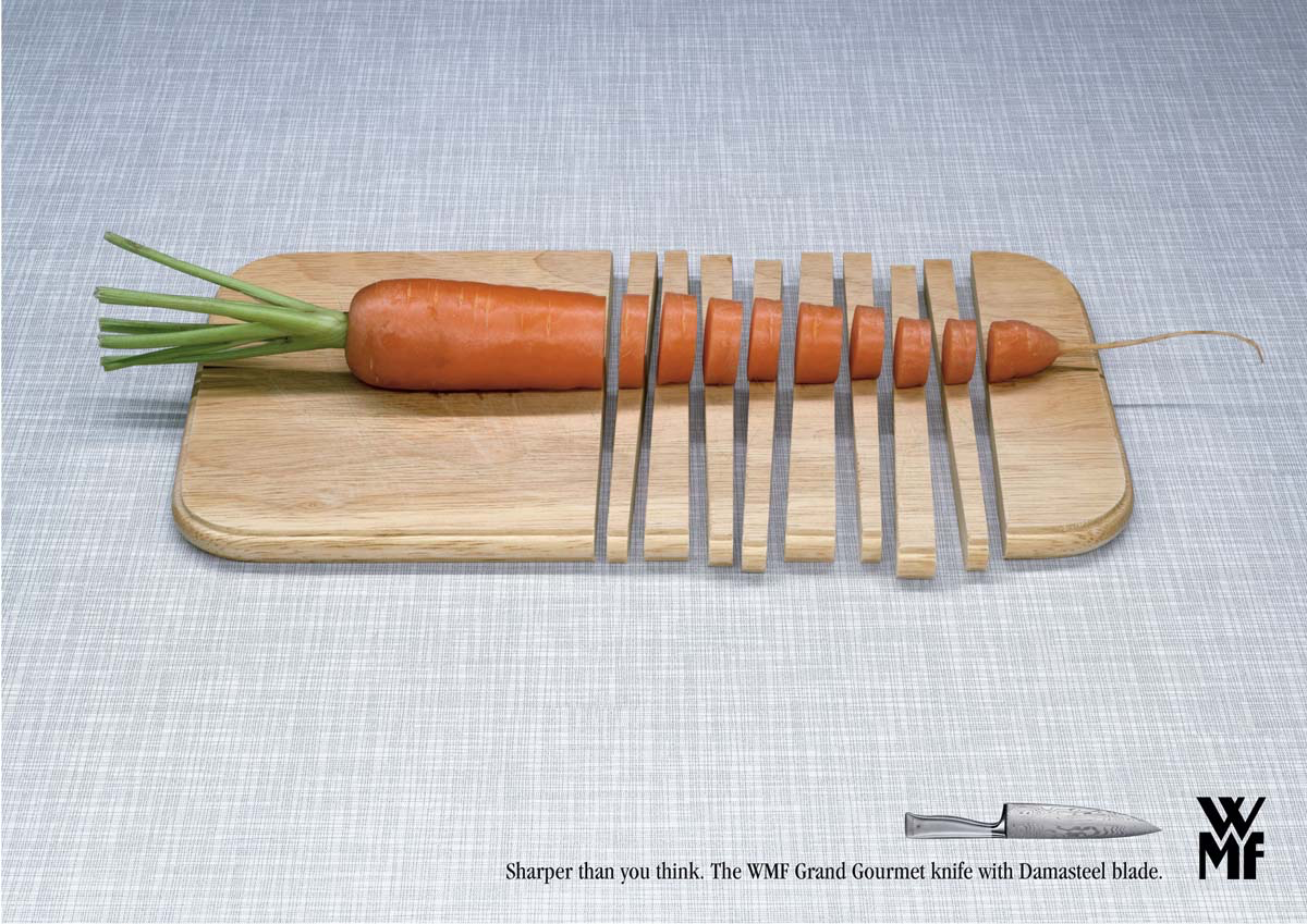
Photography basics: Depth of Field and composition
Read more: Photography basics: Depth of Field and compositionDepth of field is the range within which focusing is resolved in a photo.
Aperture has a huge affect on to the depth of field.
Changing the f-stops (f/#) of a lens will change aperture and as such the DOF.
f-stops are a just certain number which is telling you the size of the aperture. That’s how f-stop is related to aperture (and DOF).
If you increase f-stops, it will increase DOF, the area in focus (and decrease the aperture). On the other hand, decreasing the f-stop it will decrease DOF (and increase the aperture).
The red cone in the figure is an angular representation of the resolution of the system. Versus the dotted lines, which indicate the aperture coverage. Where the lines of the two cones intersect defines the total range of the depth of field.
This image explains why the longer the depth of field, the greater the range of clarity.

-
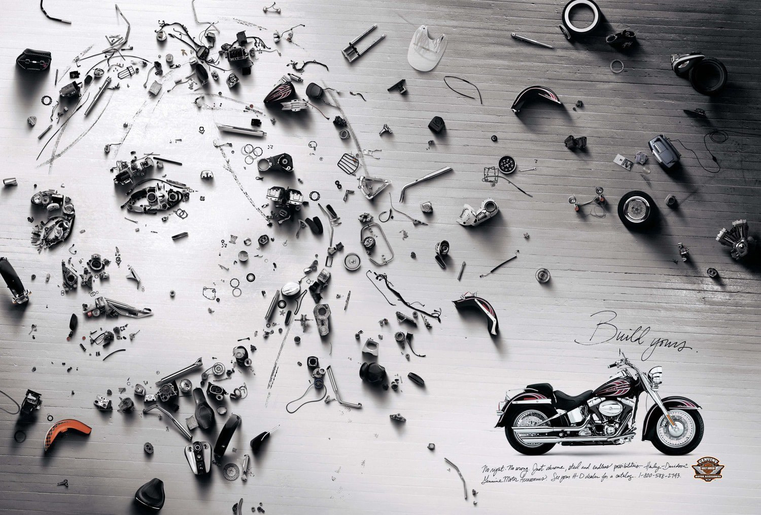
9 Best Hacks to Make a Cinematic Video with Any Camera
Read more: 9 Best Hacks to Make a Cinematic Video with Any Camerahttps://www.flexclip.com/learn/cinematic-video.html
- Frame Your Shots to Create Depth
- Create Shallow Depth of Field
- Avoid Shaky Footage and Use Flexible Camera Movements
- Properly Use Slow Motion
- Use Cinematic Lighting Techniques
- Apply Color Grading
- Use Cinematic Music and SFX
- Add Cinematic Fonts and Text Effects
- Create the Cinematic Bar at the Top and the Bottom


DESIGN
-
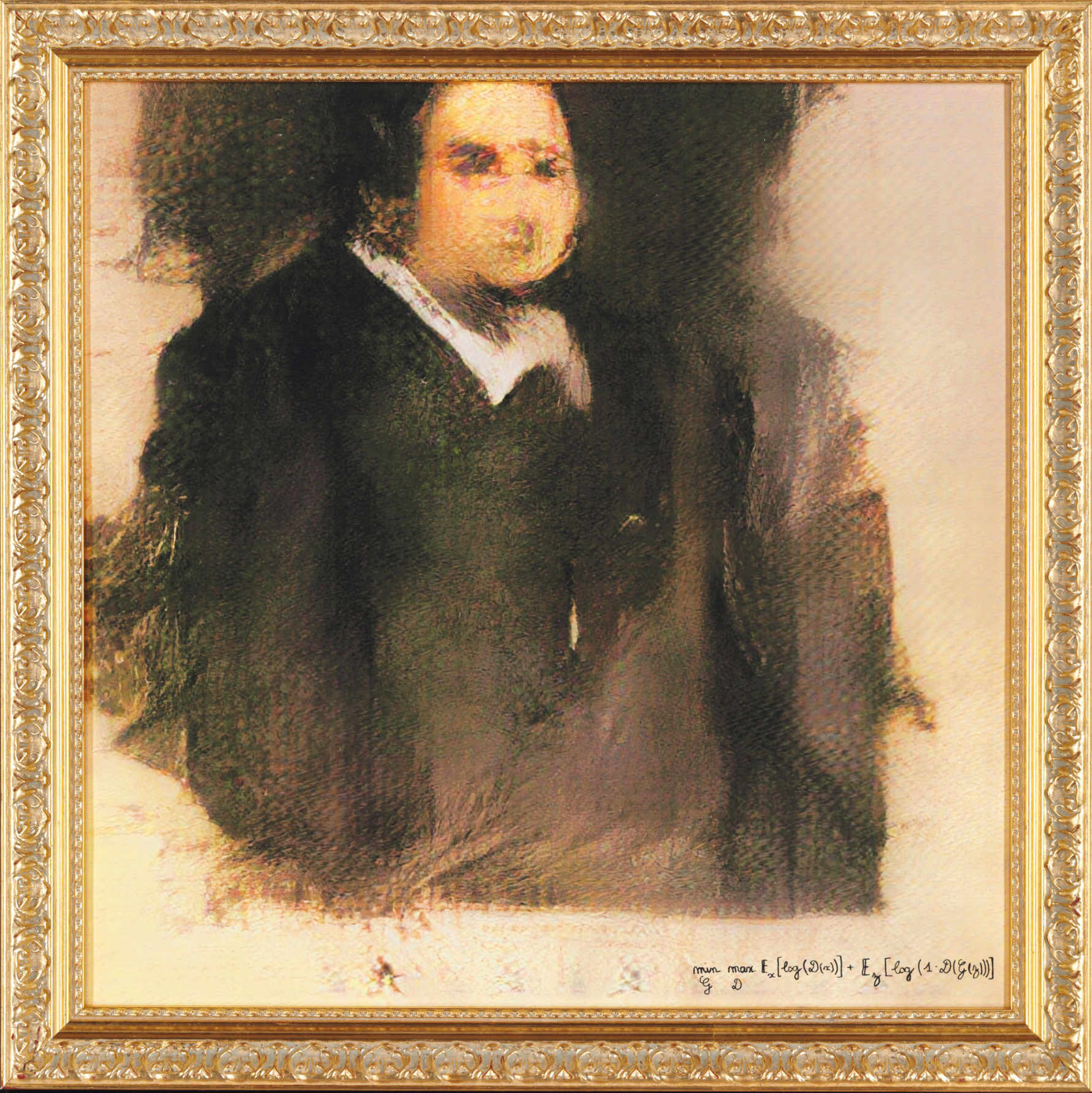
A.I. Algorithm art fetches US$432,500 at Christie auction
Read more: A.I. Algorithm art fetches US$432,500 at Christie auctionwww.ctvnews.ca/entertainment/algorithm-art-fetches-us-432-500-at-christie-s-auction-1.4150620
www.christies.com/features/A-collaboration-between-two-artists-one-human-one-a-machine-9332-1.aspx

-
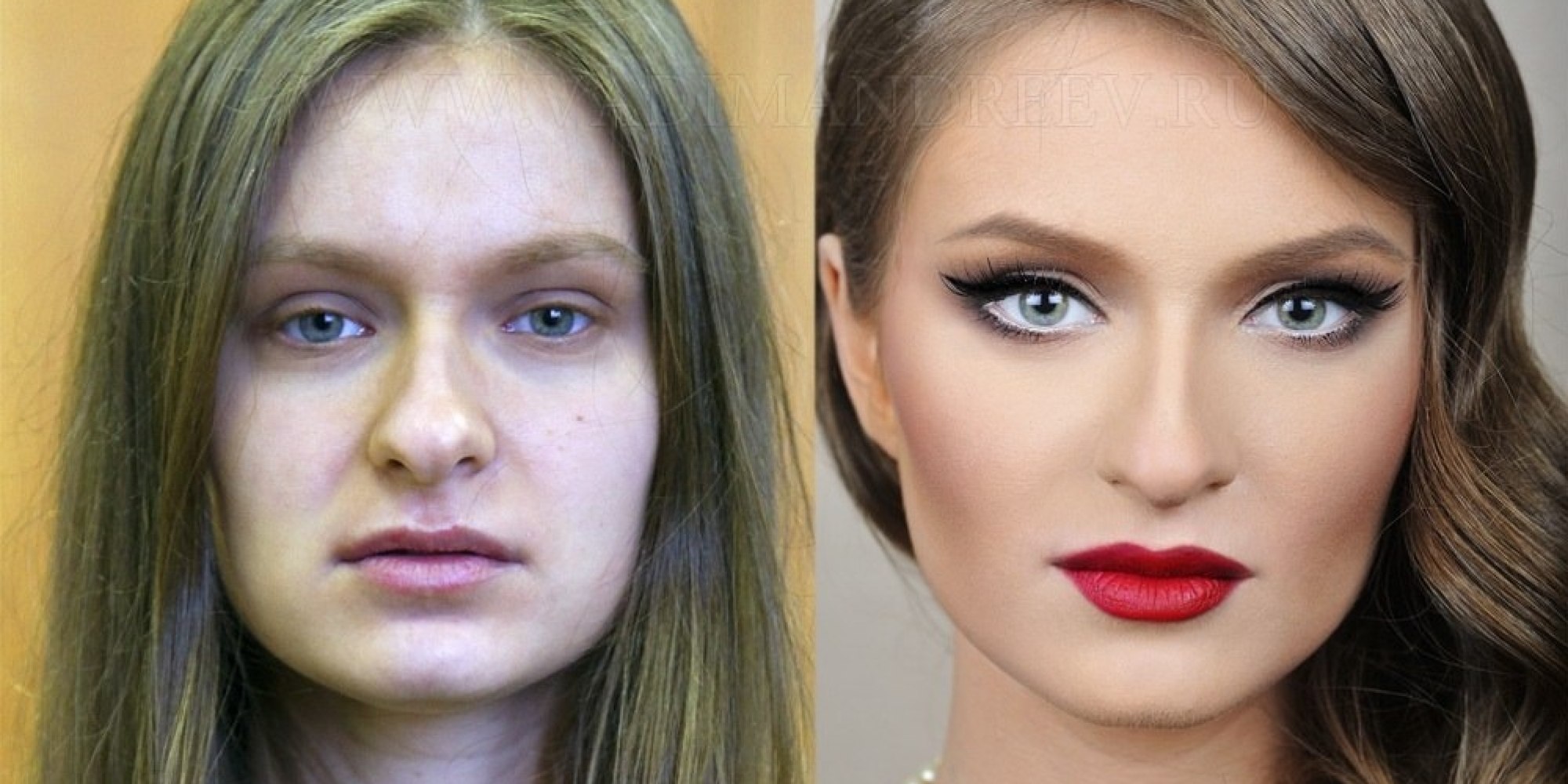
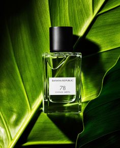
Mania Carta – Photorealistic Characters Made in Blender
Read more: Mania Carta – Photorealistic Characters Made in BlenderManiacarta is an Artist based in Tokyo, her Artworks are unique and she strive to create the best characters that have soul in the World.
https://80.lv/articles/marvelous-photorealistic-characters-made-in-blender-by-mania-carta/
https://www.instagram.com/mania_carta/


COLOR
-
Tim Kang – calibrated white light values in sRGB color space
Read more: Tim Kang – calibrated white light values in sRGB color space8bit sRGB encoded
2000K 255 139 22
2700K 255 172 89
3000K 255 184 109
3200K 255 190 122
4000K 255 211 165
4300K 255 219 178
D50 255 235 205
D55 255 243 224
D5600 255 244 227
D6000 255 249 240
D65 255 255 255
D10000 202 221 255
D20000 166 196 2558bit Rec709 Gamma 2.4
2000K 255 145 34
2700K 255 177 97
3000K 255 187 117
3200K 255 193 129
4000K 255 214 170
4300K 255 221 182
D50 255 236 208
D55 255 243 226
D5600 255 245 229
D6000 255 250 241
D65 255 255 255
D10000 204 222 255
D20000 170 199 2558bit Display P3 encoded
2000K 255 154 63
2700K 255 185 109
3000K 255 195 127
3200K 255 201 138
4000K 255 219 176
4300K 255 225 187
D50 255 239 212
D55 255 245 228
D5600 255 246 231
D6000 255 251 242
D65 255 255 255
D10000 208 223 255
D20000 175 199 25510bit Rec2020 PQ (100 nits)
2000K 520 435 273
2700K 520 466 358
3000K 520 475 384
3200K 520 480 399
4000K 520 495 446
4300K 520 500 458
D50 520 510 482
D55 520 514 497
D5600 520 514 500
D6000 520 517 509
D65 520 520 520
D10000 479 489 520
D20000 448 464 520
-
Paul Debevec, Chloe LeGendre, Lukas Lepicovsky – Jointly Optimizing Color Rendition and In-Camera Backgrounds in an RGB Virtual Production Stage
Read more: Paul Debevec, Chloe LeGendre, Lukas Lepicovsky – Jointly Optimizing Color Rendition and In-Camera Backgrounds in an RGB Virtual Production Stagehttps://arxiv.org/pdf/2205.12403.pdf
RGB LEDs vs RGBWP (RGB + lime + phospor converted amber) LEDs
Local copy:
-
Weta Digital – Manuka Raytracer and Gazebo GPU renderers – pipeline
Read more: Weta Digital – Manuka Raytracer and Gazebo GPU renderers – pipelinehttps://jo.dreggn.org/home/2018_manuka.pdf
http://www.fxguide.com/featured/manuka-weta-digitals-new-renderer/

The Manuka rendering architecture has been designed in the spirit of the classic reyes rendering architecture. In its core, reyes is based on stochastic rasterisation of micropolygons, facilitating depth of field, motion blur, high geometric complexity,and programmable shading.
This is commonly achieved with Monte Carlo path tracing, using a paradigm often called shade-on-hit, in which the renderer alternates tracing rays with running shaders on the various ray hits. The shaders take the role of generating the inputs of the local material structure which is then used bypath sampling logic to evaluate contributions and to inform what further rays to cast through the scene.
Over the years, however, the expectations have risen substantially when it comes to image quality. Computing pictures which are indistinguishable from real footage requires accurate simulation of light transport, which is most often performed using some variant of Monte Carlo path tracing. Unfortunately this paradigm requires random memory accesses to the whole scene and does not lend itself well to a rasterisation approach at all.
Manuka is both a uni-directional and bidirectional path tracer and encompasses multiple importance sampling (MIS). Interestingly, and importantly for production character skin work, it is the first major production renderer to incorporate spectral MIS in the form of a new ‘Hero Spectral Sampling’ technique, which was recently published at Eurographics Symposium on Rendering 2014.
Manuka propose a shade-before-hit paradigm in-stead and minimise I/O strain (and some memory costs) on the system, leveraging locality of reference by running pattern generation shaders before we execute light transport simulation by path sampling, “compressing” any bvh structure as needed, and as such also limiting duplication of source data.
The difference with reyes is that instead of baking colors into the geometry like in Reyes, manuka bakes surface closures. This means that light transport is still calculated with path tracing, but all texture lookups etc. are done up-front and baked into the geometry.The main drawback with this method is that geometry has to be tessellated to its highest, stable topology before shading can be evaluated properly. As such, the high cost to first pixel. Even a basic 4 vertices square becomes a much more complex model with this approach.

Manuka use the RenderMan Shading Language (rsl) for programmable shading [Pixar Animation Studios 2015], but we do not invoke rsl shaders when intersecting a ray with a surface (often called shade-on-hit). Instead, we pre-tessellate and pre-shade all the input geometry in the front end of the renderer.
This way, we can efficiently order shading computations to sup-port near-optimal texture locality, vectorisation, and parallelism. This system avoids repeated evaluation of shaders at the same surface point, and presents a minimal amount of memory to be accessed during light transport time. An added benefit is that the acceleration structure for ray tracing (abounding volume hierarchy, bvh) is built once on the final tessellated geometry, which allows us to ray trace more efficiently than multi-level bvhs and avoids costly caching of on-demand tessellated micropolygons and the associated scheduling issues.For the shading reasons above, in terms of AOVs, the studio approach is to succeed at combining complex shading with ray paths in the render rather than pass a multi-pass render to compositing.
For the Spectral Rendering component. The light transport stage is fully spectral, using a continuously sampled wavelength which is traced with each path and used to apply the spectral camera sensitivity of the sensor. This allows for faithfully support any degree of observer metamerism as the camera footage they are intended to match as well as complex materials which require wavelength dependent phenomena such as diffraction, dispersion, interference, iridescence, or chromatic extinction and Rayleigh scattering in participating media.
As opposed to the original reyes paper, we use bilinear interpolation of these bsdf inputs later when evaluating bsdfs per pathv ertex during light transport4. This improves temporal stability of geometry which moves very slowly with respect to the pixel raster
In terms of the pipeline, everything rendered at Weta was already completely interwoven with their deep data pipeline. Manuka very much was written with deep data in mind. Here, Manuka not so much extends the deep capabilities, rather it fully matches the already extremely complex and powerful setup Weta Digital already enjoy with RenderMan. For example, an ape in a scene can be selected, its ID is available and a NUKE artist can then paint in 3D say a hand and part of the way up the neutral posed ape.
We called our system Manuka, as a respectful nod to reyes: we had heard a story froma former ILM employee about how reyes got its name from how fond the early Pixar people were of their lunches at Point Reyes, and decided to name our system after our surrounding natural environment, too. Manuka is a kind of tea tree very common in New Zealand which has very many very small leaves, in analogy to micropolygons ina tree structure for ray tracing. It also happens to be the case that Weta Digital’s main site is on Manuka Street.

-
PBR Color Reference List for Materials – by Grzegorz Baran
Read more: PBR Color Reference List for Materials – by Grzegorz Baran
“The list should be helpful for every material artist who work on PBR materials as it contains over 200 color values measured with PCE-RGB2 1002 Color Spectrometer device and presented in linear and sRGB (2.2) gamma space.
All color values, HUE and Saturation in this list come from measurements taken with PCE-RGB2 1002 Color Spectrometer device and are presented in linear and sRGB (2.2) gamma space (more info at the end of this video) I calculated Relative Luminance and Luminance values based on captured color using my own equation which takes color based luminance perception into consideration. Bare in mind that there is no ‘one’ color per substance as nothing in nature is even 100% uniform and any value in +/-10% range from these should be considered as correct one. Therefore this list should be always considered as a color reference for material’s albedos, not ulitimate and absolute truth.“
-
Photography Basics : Spectral Sensitivity Estimation Without a Camera
Read more: Photography Basics : Spectral Sensitivity Estimation Without a Camerahttps://color-lab-eilat.github.io/Spectral-sensitivity-estimation-web/
A number of problems in computer vision and related fields would be mitigated if camera spectral sensitivities were known. As consumer cameras are not designed for high-precision visual tasks, manufacturers do not disclose spectral sensitivities. Their estimation requires a costly optical setup, which triggered researchers to come up with numerous indirect methods that aim to lower cost and complexity by using color targets. However, the use of color targets gives rise to new complications that make the estimation more difficult, and consequently, there currently exists no simple, low-cost, robust go-to method for spectral sensitivity estimation that non-specialized research labs can adopt. Furthermore, even if not limited by hardware or cost, researchers frequently work with imagery from multiple cameras that they do not have in their possession.
To provide a practical solution to this problem, we propose a framework for spectral sensitivity estimation that not only does not require any hardware (including a color target), but also does not require physical access to the camera itself. Similar to other work, we formulate an optimization problem that minimizes a two-term objective function: a camera-specific term from a system of equations, and a universal term that bounds the solution space.
Different than other work, we utilize publicly available high-quality calibration data to construct both terms. We use the colorimetric mapping matrices provided by the Adobe DNG Converter to formulate the camera-specific system of equations, and constrain the solutions using an autoencoder trained on a database of ground-truth curves. On average, we achieve reconstruction errors as low as those that can arise due to manufacturing imperfections between two copies of the same camera. We provide predicted sensitivities for more than 1,000 cameras that the Adobe DNG Converter currently supports, and discuss which tasks can become trivial when camera responses are available.


LIGHTING
-
HDRI Median Cut plugin
Read more: HDRI Median Cut pluginwww.hdrlabs.com/picturenaut/plugins.html

Note. The Median Cut algorithm is typically used for color quantization, which involves reducing the number of colors in an image while preserving its visual quality. It doesn’t directly provide a way to identify the brightest areas in an image. However, if you’re interested in identifying the brightest areas, you might want to look into other methods like thresholding, histogram analysis, or edge detection, through openCV for example.
Here is an openCV example:
# bottom left coordinates = 0,0 import numpy as np import cv2 # Load the HDR or EXR image image = cv2.imread('your_image_path.exr', cv2.IMREAD_UNCHANGED) # Load as-is without modification # Calculate the luminance from the HDR channels (assuming RGB format) luminance = np.dot(image[..., :3], [0.299, 0.587, 0.114]) # Set a threshold value based on estimated EV threshold_value = 2.4 # Estimated threshold value based on 4.8 EV # Apply the threshold to identify bright areas # Theluminancearray contains the calculated luminance values for each pixel in the image. # Thethreshold_valueis a user-defined value that represents a cutoff point, separating "bright" and "dark" areas in terms of perceived luminance.thresholded = (luminance > threshold_value) * 255 # Convert the thresholded image to uint8 for contour detection thresholded = thresholded.astype(np.uint8) # Find contours of the bright areas contours, _ = cv2.findContours(thresholded, cv2.RETR_EXTERNAL, cv2.CHAIN_APPROX_SIMPLE) # Create a list to store the bounding boxes of bright areas bright_areas = [] # Iterate through contours and extract bounding boxes for contour in contours: x, y, w, h = cv2.boundingRect(contour) # Adjust y-coordinate based on bottom-left origin y_bottom_left_origin = image.shape[0] - (y + h) bright_areas.append((x, y_bottom_left_origin, x + w, y_bottom_left_origin + h)) # Store as (x1, y1, x2, y2) # Print the identified bright areas print("Bright Areas (x1, y1, x2, y2):") for area in bright_areas: print(area)More details
Luminance and Exposure in an EXR Image:
- An EXR (Extended Dynamic Range) image format is often used to store high dynamic range (HDR) images that contain a wide range of luminance values, capturing both dark and bright areas.
- Luminance refers to the perceived brightness of a pixel in an image. In an RGB image, luminance is often calculated using a weighted sum of the red, green, and blue channels, where different weights are assigned to each channel to account for human perception.
- In an EXR image, the pixel values can represent radiometrically accurate scene values, including actual radiance or irradiance levels. These values are directly related to the amount of light emitted or reflected by objects in the scene.
The luminance line is calculating the luminance of each pixel in the image using a weighted sum of the red, green, and blue channels. The three float values [0.299, 0.587, 0.114] are the weights used to perform this calculation.
These weights are based on the concept of luminosity, which aims to approximate the perceived brightness of a color by taking into account the human eye’s sensitivity to different colors. The values are often derived from the NTSC (National Television System Committee) standard, which is used in various color image processing operations.
Here’s the breakdown of the float values:
- 0.299: Weight for the red channel.
- 0.587: Weight for the green channel.
- 0.114: Weight for the blue channel.
The weighted sum of these channels helps create a grayscale image where the pixel values represent the perceived brightness. This technique is often used when converting a color image to grayscale or when calculating luminance for certain operations, as it takes into account the human eye’s sensitivity to different colors.
For the threshold, remember that the exact relationship between EV values and pixel values can depend on the tone-mapping or normalization applied to the HDR image, as well as the dynamic range of the image itself.
To establish a relationship between exposure and the threshold value, you can consider the relationship between linear and logarithmic scales:
- Linear and Logarithmic Scales:
- Exposure values in an EXR image are often represented in logarithmic scales, such as EV (exposure value). Each increment in EV represents a doubling or halving of the amount of light captured.
- Threshold values for luminance thresholding are usually linear, representing an actual luminance level.
- Conversion Between Scales:
- To establish a mathematical relationship, you need to convert between the logarithmic exposure scale and the linear threshold scale.
- One common method is to use a power function. For instance, you can use a power function to convert EV to a linear intensity value.
threshold_value = base_value * (2 ** EV)Here,
EVis the exposure value,base_valueis a scaling factor that determines the relationship between EV and threshold_value, and2 ** EVis used to convert the logarithmic EV to a linear intensity value. - Choosing the Base Value:
- The
base_valuefactor should be determined based on the dynamic range of your EXR image and the specific luminance values you are dealing with. - You may need to experiment with different values of
base_valueto achieve the desired separation of bright areas from the rest of the image.
- The
Let’s say you have an EXR image with a dynamic range of 12 EV, which is a common range for many high dynamic range images. In this case, you want to set a threshold value that corresponds to a certain number of EV above the middle gray level (which is often considered to be around 0.18).
Here’s an example of how you might determine a
base_valueto achieve this:# Define the dynamic range of the image in EV dynamic_range = 12 # Choose the desired number of EV above middle gray for thresholding desired_ev_above_middle_gray = 2 # Calculate the threshold value based on the desired EV above middle gray threshold_value = 0.18 * (2 ** (desired_ev_above_middle_gray / dynamic_range)) print("Threshold Value:", threshold_value) -
Gamma correction
Read more: Gamma correction

http://www.normankoren.com/makingfineprints1A.html#Gammabox
https://en.wikipedia.org/wiki/Gamma_correction
http://www.photoscientia.co.uk/Gamma.htm
https://www.w3.org/Graphics/Color/sRGB.html
http://www.eizoglobal.com/library/basics/lcd_display_gamma/index.html
https://forum.reallusion.com/PrintTopic308094.aspx
Basically, gamma is the relationship between the brightness of a pixel as it appears on the screen, and the numerical value of that pixel. Generally Gamma is just about defining relationships.
Three main types:
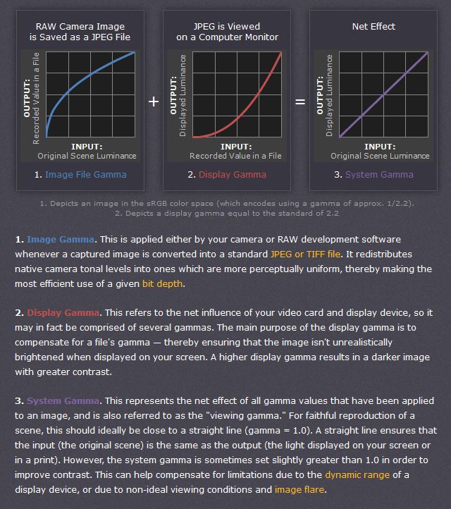
– Image Gamma encoded in images
– Display Gammas encoded in hardware and/or viewing time
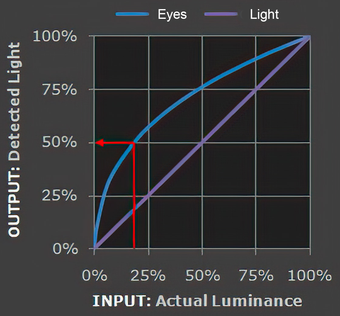
– System or Viewing Gamma which is the net effect of all gammas when you look back at a final image. In theory this should flatten back to 1.0 gamma.Our eyes, different camera or video recorder devices do not correctly capture luminance. (they are not linear)
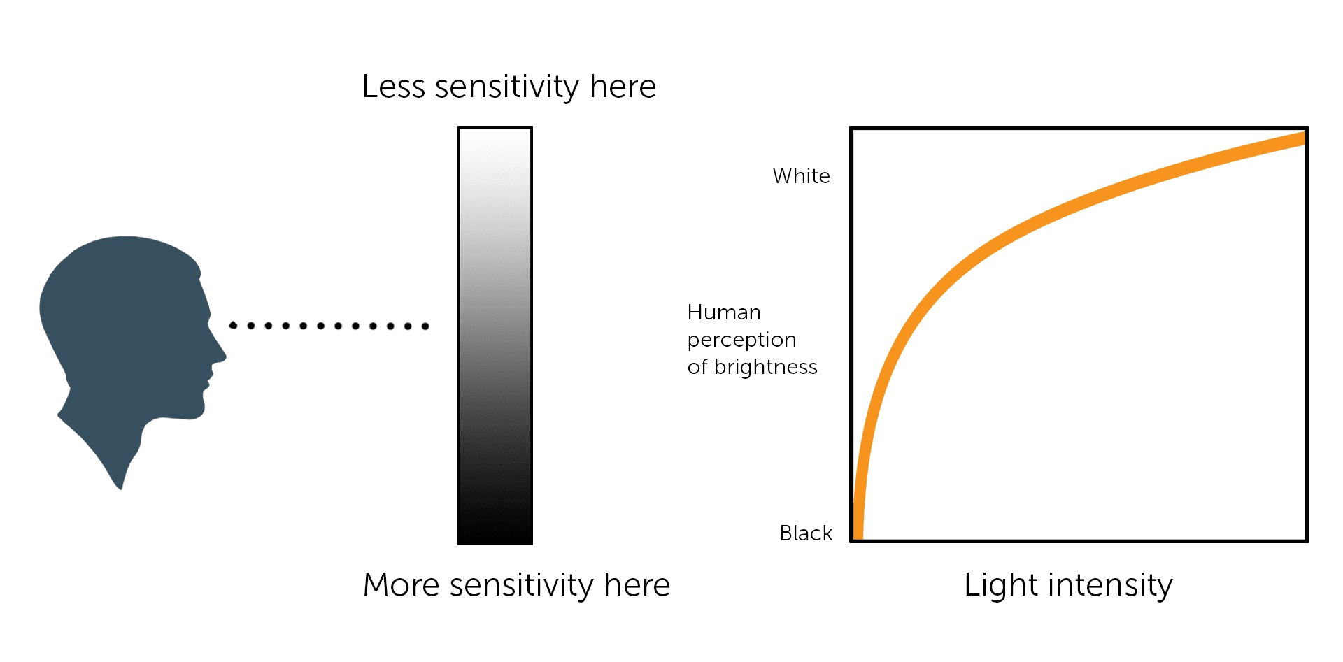
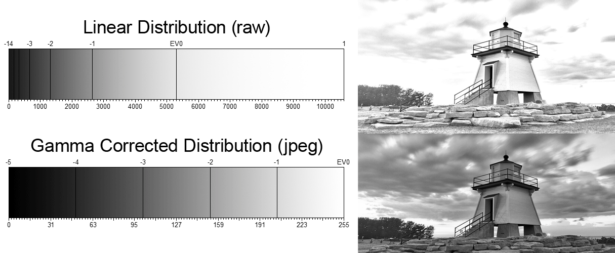
Different display devices (monitor, phone screen, TV) do not display luminance correctly neither. So, one needs to correct them, therefore the gamma correction function.The human perception of brightness, under common illumination conditions (not pitch black nor blindingly bright), follows an approximate power function (note: no relation to the gamma function), with greater sensitivity to relative differences between darker tones than between lighter ones, consistent with the Stevens’ power law for brightness perception. If images are not gamma-encoded, they allocate too many bits or too much bandwidth to highlights that humans cannot differentiate, and too few bits or too little bandwidth to shadow values that humans are sensitive to and would require more bits/bandwidth to maintain the same visual quality.
https://blog.amerlux.com/4-things-architects-should-know-about-lumens-vs-perceived-brightness/
cones manage color receptivity, rods determine how large our pupils should be. The larger (more dilated) our pupils are, the more light enters our eyes. In dark situations, our rods dilate our pupils so we can see better. This impacts how we perceive brightness.
https://www.cambridgeincolour.com/tutorials/gamma-correction.htm
A gamma encoded image has to have “gamma correction” applied when it is viewed — which effectively converts it back into light from the original scene. In other words, the purpose of gamma encoding is for recording the image — not for displaying the image. Fortunately this second step (the “display gamma”) is automatically performed by your monitor and video card. The following diagram illustrates how all of this fits together:
Display gamma
The display gamma can be a little confusing because this term is often used interchangeably with gamma correction, since it corrects for the file gamma. This is the gamma that you are controlling when you perform monitor calibration and adjust your contrast setting. Fortunately, the industry has converged on a standard display gamma of 2.2, so one doesn’t need to worry about the pros/cons of different values.Gamma encoding of images is used to optimize the usage of bits when encoding an image, or bandwidth used to transport an image, by taking advantage of the non-linear manner in which humans perceive light and color. Human response to luminance is also biased. Especially sensible to dark areas.
Thus, the human visual system has a non-linear response to the power of the incoming light, so a fixed increase in power will not have a fixed increase in perceived brightness.
We perceive a value as half bright when it is actually 18% of the original intensity not 50%. As such, our perception is not linear.You probably already know that a pixel can have any ‘value’ of Red, Green, and Blue between 0 and 255, and you would therefore think that a pixel value of 127 would appear as half of the maximum possible brightness, and that a value of 64 would represent one-quarter brightness, and so on. Well, that’s just not the case.
Pixar Color Management
https://renderman.pixar.com/color-management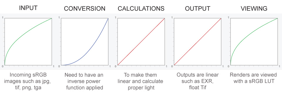
– Why do we need linear gamma?
Because light works linearly and therefore only works properly when it lights linear values.– Why do we need to view in sRGB?
Because the resulting linear image in not suitable for viewing, but contains all the proper data. Pixar’s IT viewer can compensate by showing the rendered image through a sRGB look up table (LUT), which is identical to what will be the final image after the sRGB gamma curve is applied in post.This would be simple enough if every software would play by the same rules, but they don’t. In fact, the default gamma workflow for many 3D software is incorrect. This is where the knowledge of a proper imaging workflow comes in to save the day.
Cathode-ray tubes have a peculiar relationship between the voltage applied to them, and the amount of light emitted. It isn’t linear, and in fact it follows what’s called by mathematicians and other geeks, a ‘power law’ (a number raised to a power). The numerical value of that power is what we call the gamma of the monitor or system.
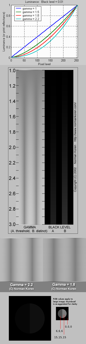
Thus. Gamma describes the nonlinear relationship between the pixel levels in your computer and the luminance of your monitor (the light energy it emits) or the reflectance of your prints. The equation is,
Luminance = C * value^gamma + black level
– C is set by the monitor Contrast control.
– Value is the pixel level normalized to a maximum of 1. For an 8 bit monitor with pixel levels 0 – 255, value = (pixel level)/255.
– Black level is set by the (misnamed) monitor Brightness control. The relationship is linear if gamma = 1. The chart illustrates the relationship for gamma = 1, 1.5, 1.8 and 2.2 with C = 1 and black level = 0.
Gamma affects middle tones; it has no effect on black or white. If gamma is set too high, middle tones appear too dark. Conversely, if it’s set too low, middle tones appear too light.
The native gamma of monitors– the relationship between grid voltage and luminance– is typically around 2.5, though it can vary considerably. This is well above any of the display standards, so you must be aware of gamma and correct it.
A display gamma of 2.2 is the de facto standard for the Windows operating system and the Internet-standard sRGB color space.
The old standard for Mcintosh and prepress file interchange is 1.8. It is now 2.2 as well.
Video cameras have gammas of approximately 0.45– the inverse of 2.2. The viewing or system gamma is the product of the gammas of all the devices in the system– the image acquisition device (film+scanner or digital camera), color lookup table (LUT), and monitor. System gamma is typically between 1.1 and 1.5. Viewing flare and other factor make images look flat at system gamma = 1.0.
Most laptop LCD screens are poorly suited for critical image editing because gamma is extremely sensitive to viewing angle.
More about screens
https://www.cambridgeincolour.com/tutorials/gamma-correction.htm
CRT Monitors. Due to an odd bit of engineering luck, the native gamma of a CRT is 2.5 — almost the inverse of our eyes. Values from a gamma-encoded file could therefore be sent straight to the screen and they would automatically be corrected and appear nearly OK. However, a small gamma correction of ~1/1.1 needs to be applied to achieve an overall display gamma of 2.2. This is usually already set by the manufacturer’s default settings, but can also be set during monitor calibration.
LCD Monitors. LCD monitors weren’t so fortunate; ensuring an overall display gamma of 2.2 often requires substantial corrections, and they are also much less consistent than CRT’s. LCDs therefore require something called a look-up table (LUT) in order to ensure that input values are depicted using the intended display gamma (amongst other things). See the tutorial on monitor calibration: look-up tables for more on this topic.
About black level (brightness). Your monitor’s brightness control (which should actually be called black level) can be adjusted using the mostly black pattern on the right side of the chart. This pattern contains two dark gray vertical bars, A and B, which increase in luminance with increasing gamma. (If you can’t see them, your black level is way low.) The left bar (A) should be just above the threshold of visibility opposite your chosen gamma (2.2 or 1.8)– it should be invisible where gamma is lower by about 0.3. The right bar (B) should be distinctly visible: brighter than (A), but still very dark. This chart is only for monitors; it doesn’t work on printed media.
The 1.8 and 2.2 gray patterns at the bottom of the image represent a test of monitor quality and calibration. If your monitor is functioning properly and calibrated to gamma = 2.2 or 1.8, the corresponding pattern will appear smooth neutral gray when viewed from a distance. Any waviness, irregularity, or color banding indicates incorrect monitor calibration or poor performance.
Another test to see whether one’s computer monitor is properly hardware adjusted and can display shadow detail in sRGB images properly, they should see the left half of the circle in the large black square very faintly but the right half should be clearly visible. If not, one can adjust their monitor’s contrast and/or brightness setting. This alters the monitor’s perceived gamma. The image is best viewed against a black background.
This procedure is not suitable for calibrating or print-proofing a monitor. It can be useful for making a monitor display sRGB images approximately correctly, on systems in which profiles are not used (for example, the Firefox browser prior to version 3.0 and many others) or in systems that assume untagged source images are in the sRGB colorspace.
On some operating systems running the X Window System, one can set the gamma correction factor (applied to the existing gamma value) by issuing the command xgamma -gamma 0.9 for setting gamma correction factor to 0.9, and xgamma for querying current value of that factor (the default is 1.0). In OS X systems, the gamma and other related screen calibrations are made through the System Preference
https://www.kinematicsoup.com/news/2016/6/15/gamma-and-linear-space-what-they-are-how-they-differ
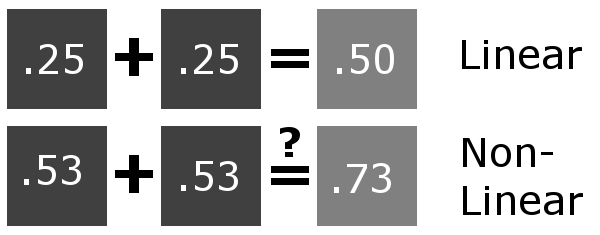
Linear color space means that numerical intensity values correspond proportionally to their perceived intensity. This means that the colors can be added and multiplied correctly. A color space without that property is called ”non-linear”. Below is an example where an intensity value is doubled in a linear and a non-linear color space. While the corresponding numerical values in linear space are correct, in the non-linear space (gamma = 0.45, more on this later) we can’t simply double the value to get the correct intensity.
The need for gamma arises for two main reasons: The first is that screens have been built with a non-linear response to intensity. The other is that the human eye can tell the difference between darker shades better than lighter shades. This means that when images are compressed to save space, we want to have greater accuracy for dark intensities at the expense of lighter intensities. Both of these problems are resolved using gamma correction, which is to say the intensity of every pixel in an image is put through a power function. Specifically, gamma is the name given to the power applied to the image.
CRT screens, simply by how they work, apply a gamma of around 2.2, and modern LCD screens are designed to mimic that behavior. A gamma of 2.2, the reciprocal of 0.45, when applied to the brightened images will darken them, leaving the original image.
-
ICLight – Krea and ComfyUI light editing
Read more: ICLight – Krea and ComfyUI light editing
https://drive.google.com/drive/folders/16Aq1mqZKP-h8vApaN4FX5at3acidqPUv
https://github.com/lllyasviel/IC-Light
https://generativematte.blogspot.com/2025/03/comfyui-ic-light-relighting-exploration.html

Workflow Local copy

-
Aputure AL-F7 – dimmable Led Video Light, CRI95+, 3200-9500K
Read more: Aputure AL-F7 – dimmable Led Video Light, CRI95+, 3200-9500KHigh CRI of ≥95
256 LEDs with 45° beam angle
3200 to 9500K variable color temperature
1 to 100% Stepless Dimming, 1500 Lux Brightness at 3.3′
LCD Info Screen. Powered by an L-series battery, D-Tap, or USB-C
Because the light has a variable color range of 3200 to 9500K, when the light is set to 5500K (daylight balanced) both sets of LEDs are on at full, providing the maximum brightness from this fixture when compared to using the light at 3200 or 9500K.
The LCD screen provides information on the fixture’s output as well as the charge state of the battery. The screen also indicates whether the adjustment knob is controlling brightness or color temperature. To switch from brightness to CCT or CCT to brightness, just apply a short press to the adjustment knob.
The included cold shoe ball joint adapter enables mounting the light to your camera’s accessory shoe via the 1/4″-20 threaded hole on the fixture. In addition, the bottom of the cold shoe foot features a 3/8″-16 threaded hole, and includes a 3/8″-16 to 1/4″-20 reducing bushing.


COLLECTIONS
| Featured AI
| Design And Composition
| Explore posts
POPULAR SEARCHES
unreal | pipeline | virtual production | free | learn | photoshop | 360 | macro | google | nvidia | resolution | open source | hdri | real-time | photography basics | nuke
FEATURED POSTS
-
The CG Career YouTube channel is live!
-
AI Data Laundering: How Academic and Nonprofit Researchers Shield Tech Companies from Accountability
-
Ross Pettit on The Agile Manager – How tech firms went for prioritizing cash flow instead of talent
-
VFX pipeline – Render Wall management topics
-
Photography basics: Solid Angle measures
-
Black Body color aka the Planckian Locus curve for white point eye perception
-
Free fonts
-
UV maps
Social Links
DISCLAIMER – Links and images on this website may be protected by the respective owners’ copyright. All data submitted by users through this site shall be treated as freely available to share.
