


COMPOSITION


DESIGN
-
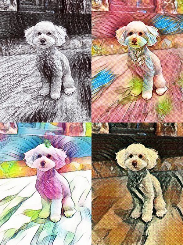
Cosmic Motors book by Daniel Simon
Read more: Cosmic Motors book by Daniel Simonhttp://danielsimon.com/cosmic-motors-the-book/
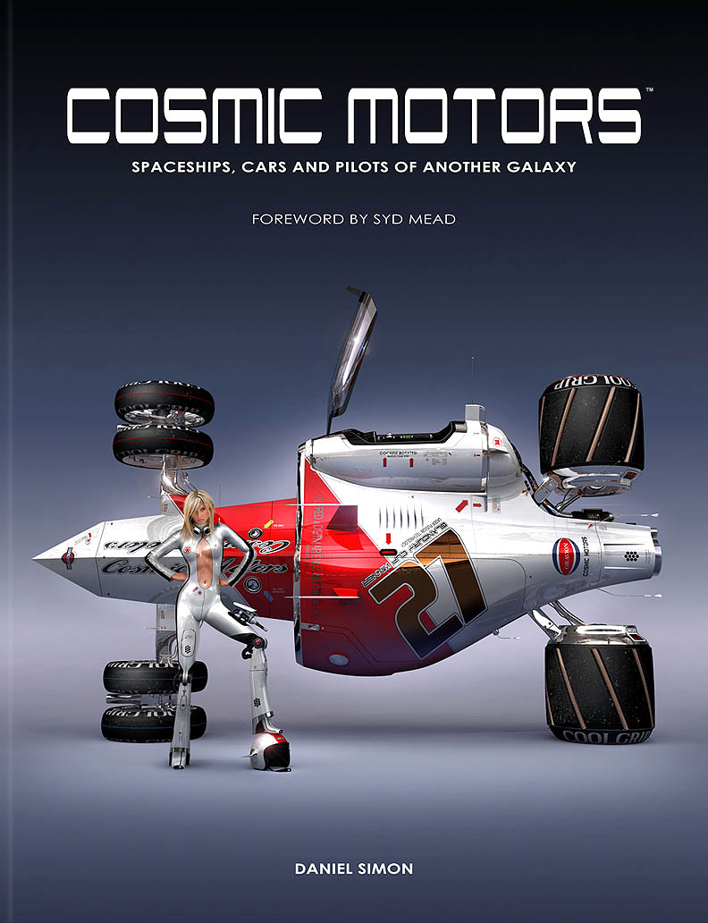
Book Cover Cosmic Motors, Copyright by Cosmic Motors LLC / Daniel Simon www.danielsimon.com


COLOR
-
HDR and Color
Read more: HDR and Colorhttps://www.soundandvision.com/content/nits-and-bits-hdr-and-color
In HD we often refer to the range of available colors as a color gamut. Such a color gamut is typically plotted on a two-dimensional diagram, called a CIE chart, as shown in at the top of this blog. Each color is characterized by its x/y coordinates.

Good enough for government work, perhaps. But for HDR, with its higher luminance levels and wider color, the gamut becomes three-dimensional.

For HDR the color gamut therefore becomes a characteristic we now call the color volume. It isn’t easy to show color volume on a two-dimensional medium like the printed page or a computer screen, but one method is shown below. As the luminance becomes higher, the picture eventually turns to white. As it becomes darker, it fades to black. The traditional color gamut shown on the CIE chart is simply a slice through this color volume at a selected luminance level, such as 50%.
Three different color volumes—we still refer to them as color gamuts though their third dimension is important—are currently the most significant. The first is BT.709 (sometimes referred to as Rec.709), the color gamut used for pre-UHD/HDR formats, including standard HD.
The largest is known as BT.2020; it encompasses (roughly) the range of colors visible to the human eye (though ET might find it insufficient!).
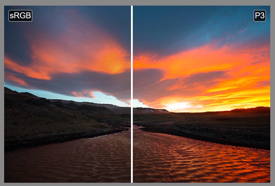
Between these two is the color gamut used in digital cinema, known as DCI-P3.

sRGB

D65

-
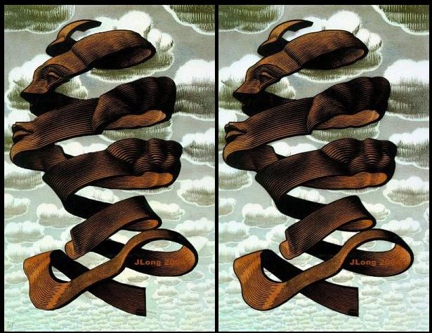
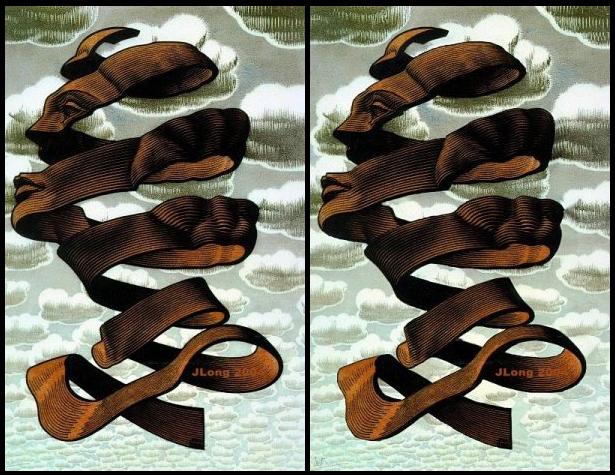
Space bodies’ components and light spectroscopy
Read more: Space bodies’ components and light spectroscopywww.plutorules.com/page-111-space-rocks.html
This help’s us understand the composition of components in/on solar system bodies.
Dips in the observed light spectrum, also known as, lines of absorption occur as gasses absorb energy from light at specific points along the light spectrum.
These dips or darkened zones (lines of absorption) leave a finger print which identify elements and compounds.
In this image the dark absorption bands appear as lines of emission which occur as the result of emitted not reflected (absorbed) light.
Lines of absorption
 Lines of emission


-
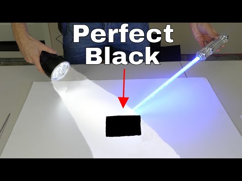
The Color of Infinite Temperature
Read more: The Color of Infinite TemperatureThis is the color of something infinitely hot.

Of course you’d instantly be fried by gamma rays of arbitrarily high frequency, but this would be its spectrum in the visible range.
johncarlosbaez.wordpress.com/2022/01/16/the-color-of-infinite-temperature/
This is also the color of a typical neutron star. They’re so hot they look the same.
It’s also the color of the early Universe!This was worked out by David Madore.

The color he got is sRGB(148,177,255).
www.htmlcsscolor.com/hex/94B1FFAnd according to the experts who sip latte all day and make up names for colors, this color is called ‘Perano’.
-
THOMAS MANSENCAL – The Apparent Simplicity of RGB Rendering
Read more: THOMAS MANSENCAL – The Apparent Simplicity of RGB Rendering
https://thomasmansencal.substack.com/p/the-apparent-simplicity-of-rgb-rendering
The primary goal of physically-based rendering (PBR) is to create a simulation that accurately reproduces the imaging process of electro-magnetic spectrum radiation incident to an observer. This simulation should be indistinguishable from reality for a similar observer.
Because a camera is not sensitive to incident light the same way than a human observer, the images it captures are transformed to be colorimetric. A project might require infrared imaging simulation, a portion of the electro-magnetic spectrum that is invisible to us. Radically different observers might image the same scene but the act of observing does not change the intrinsic properties of the objects being imaged. Consequently, the physical modelling of the virtual scene should be independent of the observer.
-
Colormaxxing – What if I told you that rgb(255, 0, 0) is not actually the reddest red you can have in your browser?
Read more: Colormaxxing – What if I told you that rgb(255, 0, 0) is not actually the reddest red you can have in your browser?https://karuna.dev/colormaxxing
https://webkit.org/blog-files/color-gamut/comparison.html
https://oklch.com/#70,0.1,197,100
-
colorhunt.co
Read more: colorhunt.coColor Hunt is a free and open platform for color inspiration with thousands of trendy hand-picked color palettes.


LIGHTING
-
Practical Aspects of Spectral Data and LEDs in Digital Content Production and Virtual Production – SIGGRAPH 2022
Read more: Practical Aspects of Spectral Data and LEDs in Digital Content Production and Virtual Production – SIGGRAPH 2022
Comparison to the commercial side

https://www.ecolorled.com/blog/detail/what-is-rgb-rgbw-rgbic-strip-lights
RGBW (RGB + White) LED strip uses a 4-in-1 LED chip made up of red, green, blue, and white.
RGBWW (RGB + White + Warm White) LED strip uses either a 5-in-1 LED chip with red, green, blue, white, and warm white for color mixing. The only difference between RGBW and RGBWW is the intensity of the white color. The term RGBCCT consists of RGB and CCT. CCT (Correlated Color Temperature) means that the color temperature of the led strip light can be adjusted to change between warm white and white. Thus, RGBWW strip light is another name of RGBCCT strip.
RGBCW is the acronym for Red, Green, Blue, Cold, and Warm. These 5-in-1 chips are used in supper bright smart LED lighting products
-
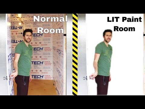
Composition and The Expressive Nature Of Light
Read more: Composition and The Expressive Nature Of Lighthttp://www.huffingtonpost.com/bill-danskin/post_12457_b_10777222.html
George Sand once said “ The artist vocation is to send light into the human heart.”

-
IES Light Profiles and editing software
Read more: IES Light Profiles and editing softwarehttp://www.derekjenson.com/3d-blog/ies-light-profiles
https://ieslibrary.com/en/browse#ies
https://leomoon.com/store/shaders/ies-lights-pack
https://docs.arnoldrenderer.com/display/a5afmug/ai+photometric+light
IES profiles are useful for creating life-like lighting, as they can represent the physical distribution of light from any light source.
The IES format was created by the Illumination Engineering Society, and most lighting manufacturers provide IES profile for the lights they manufacture.


COLLECTIONS
| Featured AI
| Design And Composition
| Explore posts
POPULAR SEARCHES
unreal | pipeline | virtual production | free | learn | photoshop | 360 | macro | google | nvidia | resolution | open source | hdri | real-time | photography basics | nuke
FEATURED POSTS
-
MiniTunes V1 – Free MP3 library app
-
N8N.io – From Zero to Your First AI Agent in 25 Minutes
-
What the Boeing 737 MAX’s crashes can teach us about production business – the effects of commoditisation
-
QR code logos
-
The Perils of Technical Debt – Understanding Its Impact on Security, Usability, and Stability
-
Free fonts
-
HDRI Median Cut plugin
-
The Public Domain Is Working Again — No Thanks To Disney
Social Links
DISCLAIMER – Links and images on this website may be protected by the respective owners’ copyright. All data submitted by users through this site shall be treated as freely available to share.
